Structured Natural Gradient Descent (ICML 2021)
July 05, 2021
More about this work [lin2021tractable]: Long talk, (Youtube) short talk, extended paper, short paper, poster
Introduction
Motivation
Many problems in optimization, search, and inference can be solved via natural-gradient descent (NGD)
Structures play an essential role in
- Preconditioners of first-order and second-order optimization, gradient-free search.
- Covariance matrices of variational Gaussian inference [opper2009variational]
Natural-gradient descent on structured parameter spaces is computationally challenging.
Limitations of existing NGD methods:
- Limited structures due to the complicated Fisher information matrix (FIM)
- Ad-hoc approximations for handling the singular FIM and cost reductions
- Inefficient and complicated natural-gradient computation
| Existing approach for rank-one covariance | Our NGD for rank-one covariance |
|---|---|
 |
 |
Our Contributions
We propose a flexible and efficient NGD method to incorporate structures via matrix Lie groups.
Our NGD method
- generalizes the exponential natural evolutionary strategy [glasmachers2010exponential]
- recovers existing Newton-like algorithms
- yields new structured 2nd-order methods and adaptive-gradient methods with group-structural invariance [lin2021structured]
- gives new NGD updates to learn structured covariances of Gaussian, Wishart and their mixtures
- is a systematic approach to incorporate a range of structures
Applications of our method:
- deep learning (structured adaptive-gradient),
- non-convex optimization (structured 2nd-order),
- evolution strategies (structured gradient-free),
- variational mixture of Gaussians (Monte Carlo gradients for structured covariance).
NGD for Optimization, Inference, and Search
A unified view for problems in optimization, inference, and search
as optimization over (variational) parametric family $q(w|\tau)$:
$$
\begin{aligned}
   \min_{ \tau \in \Omega_\tau } \mathcal{L}(\tau):= \mathrm{E}_{q(\text{w}| \tau )} \big[ \ell(\mathbf{w}) \big] + \gamma \mathrm{E}_{q(\text{w} |\tau )} \big[ \log q(w|\tau) \big]
\end{aligned} \tag{1}\label{1}
$$
where $\mathbf{w}$ is the decision variable, $\ell(\mathbf{w})$ is a loss function, $\Omega_\tau$ is the parameter space of $q$, and $\gamma\ge 0$ is a constant.
Using gradient descent and natural-gradient descent to solve $\eqref{1}$:
$$
\begin{aligned}
\textrm{GD: } &\tau_{t+1} \leftarrow \tau_t - \alpha \nabla_{\tau_t} \mathcal{L}(\tau) \\
\textrm{Standard NGD: } & \tau_{t+1} \leftarrow \tau_t - \beta\,\, \big[ \mathbf{F}_{\tau} (\tau_t) \big]^{-1} \nabla_{\tau_t} \mathcal{L}(\tau)
\end{aligned}
$$
where $\mathbf{F}_{\tau} (\tau_t)$ is the FIM of distribution $q(w|\tau)$ at $\tau=\tau_t$.
For an introduction to natural-gradient methods, see this blog.
Advantages of NGD:
- recovers a Newton-like update for Gaussian family
$q(\mathbf{w}|\mu,\mathbf{S})$with parameter$\tau=(\mu,\mathbf{S})$, mean$\mu$, and precision$\mathbf{S}$.$$ \begin{aligned} \mu_{t+1} & \leftarrow \mu_t - \beta \mathbf{S}_{t}^{-1} E_{q(\text{w}|\tau_t)}{ \big[ \nabla_w \ell( \mathbf{w}) \big] } \\ \mathbf{S}_{t+1} & \leftarrow (1-\beta \gamma)\mathbf{S}_t + \beta E_{q(\text{w}|\tau_t)}{ \big[ \nabla_w^2 \ell(\mathbf{w}) \big] } \end{aligned} \tag{2}\label{2} $$ - is less sensitive to parameter transformations than GD
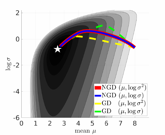
- converges faster than GD
Challenges of standard NGD:
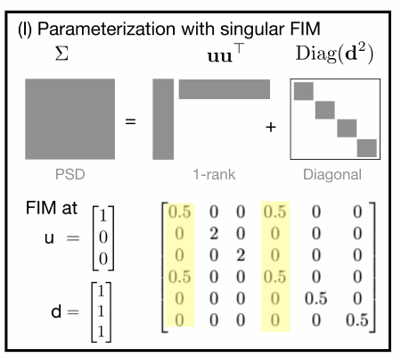
- NGD could violate parameterization constraints (e.g.,
$\mathbf{S}_{t+1}$in$\eqref{2}$may not be positive-definite) - Singular Fisher information matrix (FIM)
$\mathbf{F}_{\tau}(\tau)$of$q(w|\tau)$ - Limited precision/covariance structures
- Ad-hoc approximations for cost reductions
- Complicated and inefficient natural-gradient computation
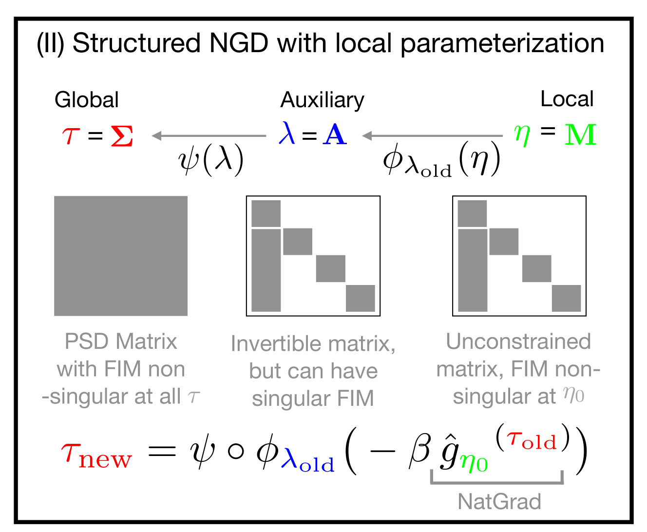
NGD using Local Parameterizations
Our method performs NGD updates in local parameter $\eta$ while maintaining structures via matrix groups in auxiliary parameter $\lambda$. This decoupling enables a tractable update that exploits the structures in auxiliary parameter spaces.
 |
When $\tau$ space has a local vector-space structure, standard NGD in $\tau$ space is a special case of our NGD, where we choose $\psi$ to be the identity map and $\phi_{\lambda_t}$ to be a linear map. |
We consider the following three kinds of parameterizations.
- Global (original) parameterization
$\tau$for$q(w|\tau)$ - New auxiliary parameterization
$\lambda$with a surjective map:$\tau= \psi(\lambda)$ - Local parameterization
$\eta$for$\lambda$at a current value$\lambda_t$with a local map:$\lambda = \phi_{\lambda_t} (\eta)$,
where$\phi_{\lambda_t}$is tight at$\lambda_t$: $\lambda_t \equiv \phi_{\lambda_t} (\eta_0)$, and we assume$\eta_0 =\mathbf{0}$to be a relative origin.
where $\hat{\mathbf{g}}_{\eta_0}^{(t)}$ is
the natural-gradient $\hat{\mathbf{g}}_{\eta_0}^{(t)}$ at $\eta_0$ tied to $\lambda_t$, which is computed by the chain rule,
$$
\begin{aligned}
        \hat{\mathbf{g}}_{\eta_0}^{(t)} &=  {\color{green}\mathbf{F}_{\eta}(\eta_0)^{-1} }
         \,\, \big[ \nabla_{\eta_0} \big[ \psi \circ \phi_{\lambda_t} (\eta) \big]
        \nabla_{\tau_t}\mathcal{L}(\tau) \big]
\end{aligned}
$$
where $\mathbf{F}_{\eta}(\eta_0)$ is the (exact) FIM for $\eta_0$ tied to $\lambda_t$.
Our method allows us to choose map $\psi \circ \phi_{\lambda_t}$ so that
the FIM $\mathbf{F}_{\eta}(\eta_0)$ is easy to inverse at $\eta_0$, which enables tractable natural-gradient
computation.
Gaussian Example with Full Precision
Notations:
$\mathrm{GL}^{p\times p}$: Invertible Matrices (General Linear Group),$\mathcal{D}^{p\times p}$: Diagonal Matrices,$\mathcal{D}_{++}^{p\times p}$: Diagonal and invertible Matrices (Diagonal Matrix Group),$\mathcal{S}_{++}^{p\times p}$: (Symmetric) positive-definite Matrices,$\mathcal{S}^{p\times p}$: Symmetric Matrices.
Consider a Gaussian family $q(w|\mu,\mathbf{S})$ with mean $\mu$ and precision $\mathbf{S}=\Sigma^{-1}$.
The global, auxiliary, and local parameterizations are:
$$
\begin{aligned}
        \tau &= \Big\{\mu \in \mathcal{R}^p, \mathbf{S} \in \mathcal{S}_{++}^{p\times p} \Big\},  & \mathbf{S}: \text{positive-definite matrix} \\
        \lambda & = \Big\{ \mu \in  \mathcal{R}^p , \mathbf{B} \in\mathrm{GL}^{p\times p} \Big\}, &\mathbf{B}: \text{ (closed, connected) matrix Lie group member}\\
        \eta &= \Big\{ \delta\in  \mathcal{R}^p, \mathbf{M} \in\mathcal{S}^{p\times p}  \Big\}, & \mathbf{M}: \text{ member in a sub-space of Lie algebra}
\end{aligned}
$$
Define $\mathbf{h}(\mathbf{M}):=\mathbf{I}+\mathbf{M}+\frac{1}{2} \mathbf{M}^2$.
Maps $\psi$ and $\phi_{\lambda_t}$ are :
$$
\begin{aligned}
        \Big\{ \begin{array}{c} \mu \\ \mathbf{S} \end{array} \Big\} = \psi(\lambda) & := \Big \{ \begin{array}{c} \mu \\ \mathbf{B}\mathbf{B}^\top \end{array} \Big \}, \\
       \Big \{ \begin{array}{c} \mu \\ \mathbf{B} \end{array} \Big \} = \phi_{\lambda_t}(\eta) & := \Big \{ \begin{array}{c} \mu_t + \mathbf{B}_t^{-T} \delta \\ \mathbf{B}_t \mathbf{h} (\mathbf{M}) \end{array} \Big \}.
\end{aligned} \tag{3}\label{3}
$$
We propose using Lie-group retraction map $\mathbf{h}()$ to
- keep natural-gradient computation tractable
- maintain numerical stability
- enable lower iteration cost compared to the matrix exponential map suggested in [glasmachers2010exponential]
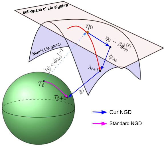
Our NGD update in $ \lambda $ space is shown below, where we assume $\eta_0=\mathbf{0}$.
$$
\begin{aligned}
  \Big\{ \begin{array}{c} \mu_{t+1} \\ \mathbf{B}_{t+1} \end{array} \Big\} = \lambda_{t+1} =
  \phi_{\lambda_t} \big( \eta_0-\beta \hat{\mathbf{g}}_{\eta_0}^{(t)} \big)
  =\Big\{ \begin{array}{c}  \mu_t - \beta \mathbf{B}_{t}^{-T} \mathbf{B}_t^{-1} \mathbf{g}_{\mu_t} \\ \mathbf{B}_t  \mathbf{h}\big(\beta \mathbf{B}_t^{-1}\mathbf{g}_{\Sigma_t} \mathbf{B}_t^{-T} \big) \end{array} \Big\}
 \end{aligned}
$$
where tractable natural-gradient $\hat{\mathbf{g}}_{\eta_0}^{(t)}$ at $\eta_0=\{\delta_0, \mathbf{M}_0\}$ tied to $\lambda_t=\{\mu_t,\mathbf{B}_t\}$ is
$$
\begin{aligned}
    \hat{\mathbf{g}}_{\eta_0}^{(t)} =
 \Big(  \begin{array}{c} \hat{\mathbf{g}}_{\delta_0}^{(t)}\\ \mathrm{vec}(  \hat{\mathbf{g}}_{M_0}^{(t)})\end{array}   \Big)
= \underbrace{  {\color{green} \Big(\begin{array}{cc} \mathbf{I}_p & 0 \\ 0 & 2 \mathbf{I}_{p^2} \end{array} \Big)^{-1}}  }_{ \text{inverse of the exact FIM } } \Big[\begin{array}{c}  \mathbf{B}_t^{-1} \mathbf{g}_{\mu_t} \\ \mathrm{vec}( -2\mathbf{B}_t^{-1} \mathbf{g}_{\Sigma_t} \mathbf{B}_t^{-T}) \end{array} \Big] \,\,\,\,& (\text{tractable: easy to inverse FIM at  } \eta_0)
\end{aligned}
$$
Note that $\mathbf{g}_\mu$ and $\mathbf{g}_{\Sigma}$ are Euclidean gradients of $\eqref{1}$ computed via Stein’s lemma [opper2009variational] [lin2019stein] :
$$
\begin{aligned}
\mathbf{g}_\mu = \nabla_{\mu}\mathcal{L}(\tau) = E_{q}{ \big[ \nabla_w \ell( \mathbf{w} ) \big] }, \,\,\,\,\,
\mathbf{g}_{\Sigma}  = \nabla_{S^{-1}}\mathcal{L}(\tau)
 = \frac{1}{2}  E_{q}{ \big[ \nabla_w^2 \ell( \mathbf{w}) \big] } - \frac{\gamma}{2} \mathbf{S}
 \end{aligned} \tag{4}\label{4}
$$
Our update on $\mathbf{S}_{t+1}=\mathbf{B}_{t+1}\mathbf{B}_{t+1}^T$ and $\mu_{t+1}$ is like update of $\eqref{2}$ as
$$
\begin{aligned}
& \mu_{t+1}   = \mu_t - \beta \mathbf{S}_{t}^{-1} E_{q(\text{w}|\tau_t)}{ \big[ \nabla_w \ell( \mathbf{w} ) \big] } \\
&\mathbf{S}_{t+1} =   \underbrace{ \overbrace{(1-\beta \gamma)\mathbf{S}_t + \beta  E_{q(w|\tau_t)}{ \big[ \nabla_w^2 \ell(\mathbf{w}) \big] }}^{\text{standard NGD on $\mathbf{S}$ }} + { \color{red} \frac{\beta^2}{2} \mathbf{G}_t \mathbf{S}_t^{-1}\mathbf{G}_t}
}_{\color{red}{\text{ RGD with retraction}}}+ O(\beta^3)
 \end{aligned}
$$
where $\mathbf{B}$ is a dense matrix in matrix group $\mathrm{GL}^{p\times p}$ and $\mathbf{G}_t := E_{q(w|\tau_t)}{ \big[ \nabla_w^2 \ell(\mathbf{w}) ] } -\gamma \mathbf{S}_t$.
The second-order term shown in red is used for the positive-definite constraint [lin2020handling] known as a retraction in Riemannian gradient descent (RGD). The higher-order term $O(\beta^3)$ will be used for structured precision matrices in the next section.
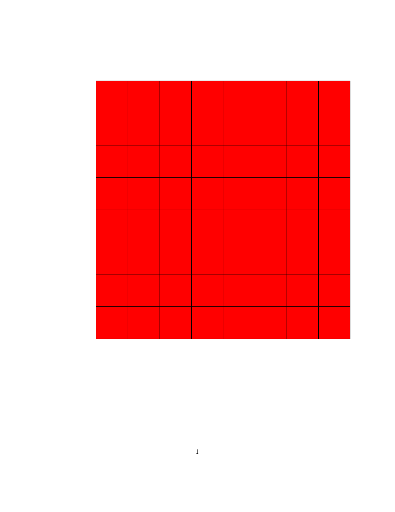
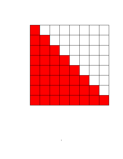
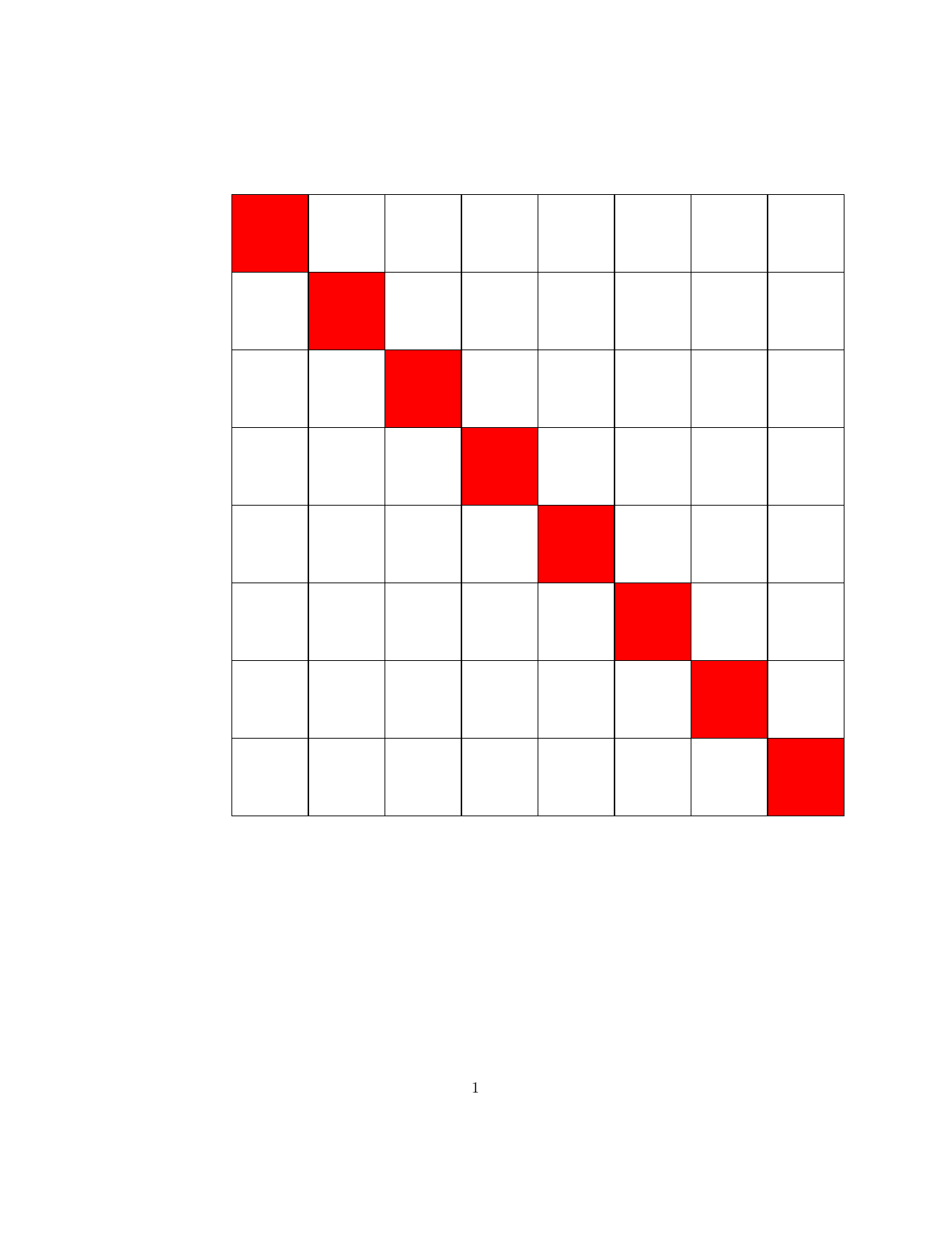
Well-known (group) structures in matrix $\mathbf{B}$ are illustrated in the following figure.
| Dense (invertible) | Triangular (Cholesky) | Diagonal (invertible) |
|---|---|---|
 |
 |
 |
Structured Gaussian with Flexible Precision
Structures in precision $\mathbf{S}$, where $\mathbf{S}=\mathbf{B}\mathbf{B}^T$ and matrix $\mathbf{B}$
is a sparse (group) member as below.
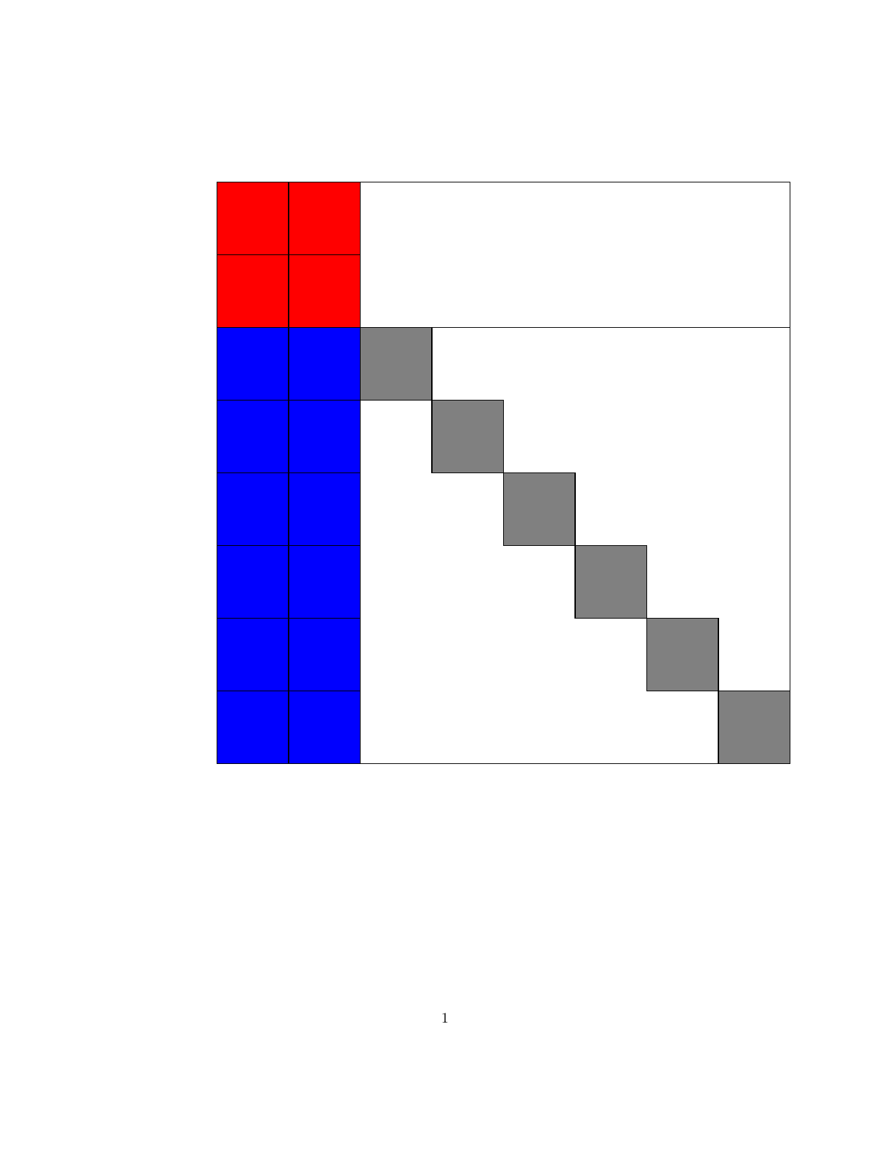
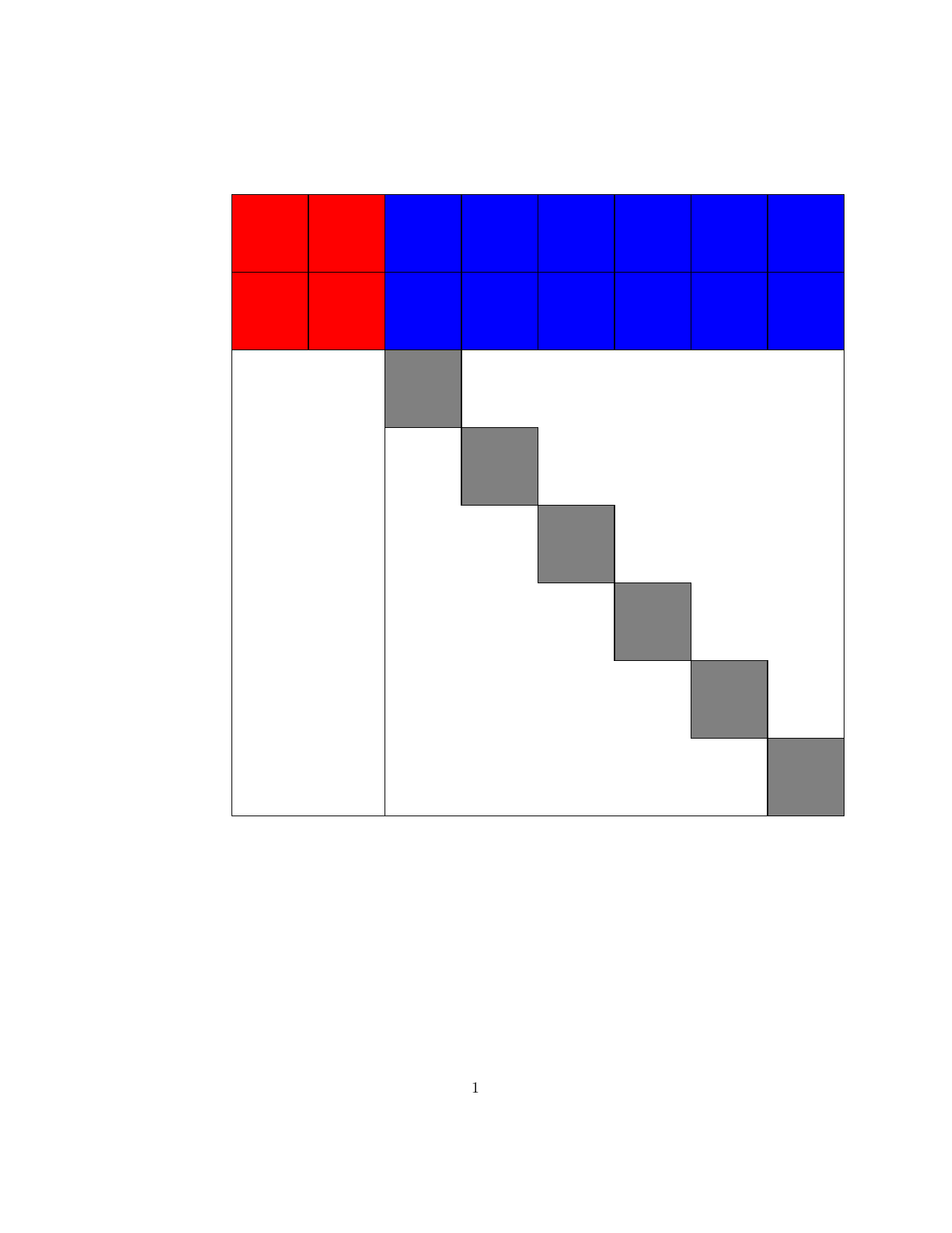
| Block lower triangular |
Block upper triangular |
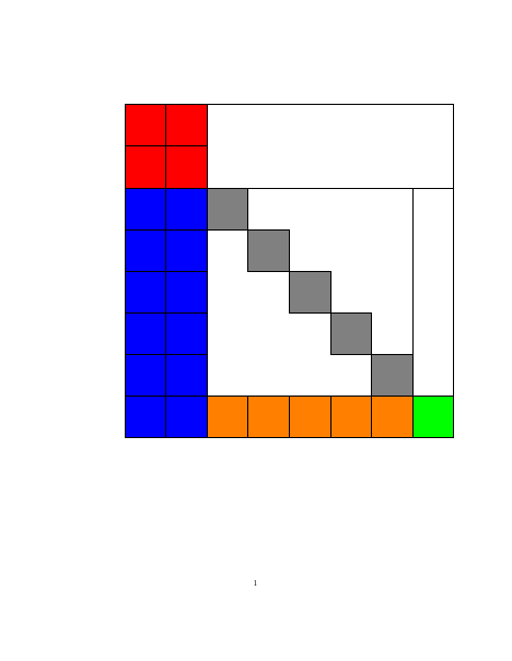
Hierarchical (lower Heisenberg) |
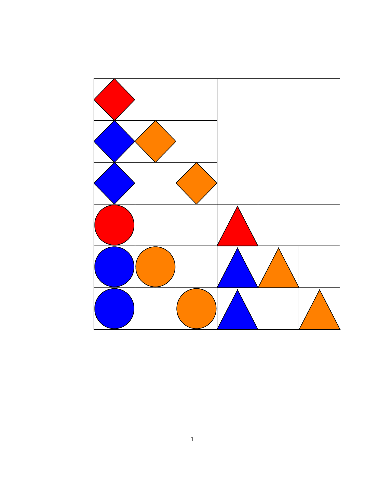
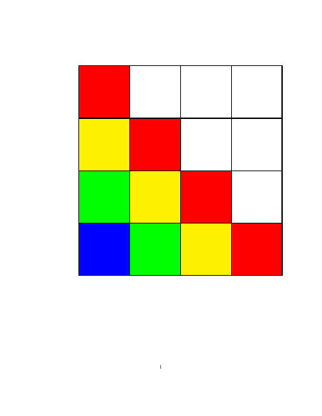
Kronecker product | Triangular-Toeplitz | Sparse Cholesky |
|---|---|---|---|---|---|
 |
 |
 |
 |
 |
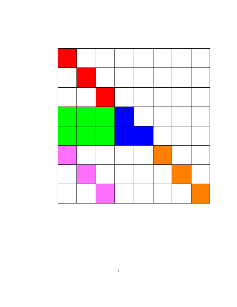 |
$\begin{bmatrix} \mathbf{B}_A & \mathbf{0} \\ \mathbf{B}_C & \mathbf{B}_D \end{bmatrix}$ |
$\begin{bmatrix} \mathbf{B}_A & \mathbf{B}_B \\ \mathbf{0} & \mathbf{B}_D \end{bmatrix}$ |
$\begin{bmatrix} \mathbf{B}_A & \mathbf{0} \\ \mathbf{B}_C & \begin{bmatrix} \mathbf{B}_{D_1} & \mathbf{0} \\ \mathbf{B}_{3} & \mathbf{B}_{4} \end{bmatrix} \end{bmatrix}$ |
$\begin{bmatrix} d & 0 \\ s & t \end{bmatrix} \otimes \begin{bmatrix} r & 0 & 0 \\ {b}_1 & {o}_1 & 0 \\ {b}_2 & 0 & {o}_2 \end{bmatrix} $ |
$\begin{bmatrix} r & 0 & 0 &0 \\ y & r & 0 & 0 \\ g & y & r & 0 \\ b & g & y & r \end{bmatrix}$ |
$\begin{bmatrix} \mathbf{B}_{D_1} & \mathbf{0} & \mathbf{0} \\ \mathbf{B}_{A} & \mathbf{B}_{B} & \mathbf{0} \\ \mathbf{B}_{D_2} & \mathbf{0} & \mathbf{B}_{D_3} \end{bmatrix}$ |
A Structured Gaussian Example:
Auxiliary parameter $\mathbf{B}$ lives in a structured space (matrix Lie group):
${\cal{B}_{\text{up}}}(k)$, a block upper-triangular sub-group of$\mathrm{GL}^{p \times p}$;
$$
\begin{aligned}
{\cal{B}_{\text{up}}}(k)  := \Big\{
\begin{bmatrix}
\mathbf{B}_A &  \mathbf{B}_B  \\
\mathbf{0} & \mathbf{B}_D
     \end{bmatrix} \Big| & \mathbf{B}_A \in \mathrm{GL}^{k \times k},\,
\mathbf{B}_D  \in{\cal D}^{(p-k) \times (p-k)}_{++}  \Big\},\,\,
\end{aligned}
$$
When
$k=0$, the space${\cal{B}_{\text{up}}}(0) = {\cal D}^{p \times p}_{++}$becomes the diagonal case. When$k=p$,${\cal{B}_{\text{up}}}(p) = \mathrm{GL}^{p\times p}$becomes the dense case.Consider a local parameter space (sub-space of Lie algebra):
${\cal{M}_{\text{up}}}(k)$.
$$
\begin{aligned}
{\cal{M}_{\text{up}}}(k):  = \Big\{
\begin{bmatrix}
\mathbf{M}_A &  \mathbf{M}_B  \\
\mathbf{0} & \mathbf{M}_D
     \end{bmatrix} \Big| &  \mathbf{M}_A \in{\cal S}^{k \times k}, \,
\mathbf{M}_D  \in{\cal D}^{(p-k) \times (p-k)} \Big\}
\end{aligned}
$$
The global, auxiliary, and local parameterizations :
$$
\begin{aligned}
      \tau &= \Big\{\mu \in \mathcal{R}^p,  \mathbf{S}=\mathbf{B} \mathbf{B}^T \in \mathcal{S}_{++}^{p\times p} | \mathbf{B} \in {\cal{B}_{\text{up}}}(k) \Big\}, \\
       \lambda & = \Big\{ \mu \in \mathcal{R}^p,  \mathbf{B} \in {\cal{B}_{\text{up}}}(k) \Big\},\\
       \eta &= \Big\{ \delta\in \mathcal{R}^p,  \mathbf{M} \in {\cal{M}_{\text{up}}}(k)   \Big\}.
\end{aligned}
$$
Maps
$\psi$and$\phi_{\lambda_t}$are defined in$\eqref{3}$. Our NGD update in the auxiliary space is shown below, where we assume $\eta_0=\mathbf{0}$.where
$\odot$is the elementwise product ,$\kappa_{\text{up}}(\mathbf{X}) \in {\cal{M}_{\text{up}}}(k)$extracts non-zero entries of${\cal{M}_{\text{up}}}(k)$from$\mathbf{X}$,$ \mathbf{C}_{\text{up}} = \begin{bmatrix} \frac{1}{2} \mathbf{J}_A & \mathbf{J}_B \\ \mathbf{0} & \frac{1}{2} \mathbf{I}_D \end{bmatrix} \in {\cal{M}_{\text{up}}}(k)$, and $\mathbf{J}$ is a matrix of ones.Note that (see [lin2021tractable] for the detail)
$ \mathbf{B}_{t+1} \in$matrix Lie group${\cal{B}_{\text{up}}}(k)$since$$ \begin{aligned} &\mathbf{h}\big(\mathbf{M}\big) \in {\cal{B}_{\text{up}}}(k) \text{ for } \mathbf{M} \in \text{Lie algebra of } {\cal{B}_{\text{up}}}(k) \,\,\,\, &(\text{by design, } \mathbf{h}(\cdot) \text{ is a Lie-group retraction}) \\ &\mathbf{B}_{t} \in {\cal{B}_{\text{up}}}(k) \,\,\,\, & (\text{by construction}) \\ &\mathbf{B}_{t+1} = \mathbf{B}_{t}\mathbf{h}\big(\mathbf{M}\big) \,\,\,\, & (\text{closed under the group product}) \end{aligned} $$$\mathbf{B}$also induces a low-rank-plus-diagonal structure in covariance matrix$\Sigma=\mathbf{S}^{-1}$, where$\mathbf{S}=\mathbf{B}\mathbf{B}^T$.
In summary, our NGD method:
- is a systematic approach to incorporate structures
- induces exact and non-singular FIMs
Applications
Structured 2nd-order Methods for Non-convex Optimization
Given an optimization problem
$$
\begin{aligned}
\min_{\mu \in \mathcal{R}^p} \ell(\mu),
 \end{aligned}\tag{5}\label{5}
$$
we formulate a new problem over Gaussian $q(\mathbf{w}|\tau)$ with structured precision, which is a special case of $\eqref{1}$ with $\gamma=1$.
$$
\begin{aligned}
   \min_{\tau \in \Omega_\tau} E_{q(w|\tau)} \big[ \ell(\mathbf{w}) \big] +  E_{q(w|\tau)} \big[ \log q(\mathbf{w}|\tau)\big],
 \end{aligned}\tag{6}\label{6}
$$
where $\mathbf{B} \in {\cal{B}_{\text{up}}}(k)$ is a block upper-triangular group member, $\tau=(\mu,\mathbf{S})$ with mean $\mu$ and precision matrix $\mathbf{S}=\mathbf{B}\mathbf{B}^T$.
Using our NGD to solve $\eqref{6}$
- gives the following update
$$ \begin{aligned} \mu_{t+1} & \leftarrow \mu_{t} - \beta \mathbf{S}_t^{-1} \mathbf{g}_{\mu_t},\\ \mathbf{B}_{t+1} & \leftarrow \mathbf{B}_t \mathbf{h} \Big( \beta \mathbf{C}_{\text{up}} \odot \kappa_{\text{up}}\big( 2 \mathbf{B}_t^{-1} \mathbf{g}_{\Sigma_t} \mathbf{B}_t^{-T} \big) \Big) \end{aligned} $$ - obtains an update to solve
$\eqref{5}$with group-structural invariance [lin2021structured]:$$ \begin{aligned} \mu_{t+1} & \leftarrow \mu_t - \beta \mathbf{S}_{t}^{-1} \nabla_{\mu_t} \ell( \mu), \\ \mathbf{B}_{t+1} & \leftarrow \mathbf{B}_t \mathbf{h} \Big( \beta \mathbf{C}_{\text{up}} \odot { \color{red}\kappa_{\text{up}}\big( \mathbf{B}_t^{-1} \nabla_{\mu_t}^2 \ell( \mu) \mathbf{B}_t^{-T} - \mathbf{I} \big)} \Big) \end{aligned}\tag{7}\label{7} $$by using$\eqref{4}$evaluated at the mean$\mu_t$$$ \begin{aligned} \mathbf{g}_{\mu_t} \approx \nabla_{\mu_t} \ell( \mu),\,\,\,\, \mathbf{g}_{\Sigma_t} \approx \frac{1}{2} \big[ \nabla_{\mu_t}^2 \ell( \mu) - \mathbf{S}_t\big]. \end{aligned}\tag{8}\label{8} $$where $\Sigma=\mathbf{S}^{-1}$ is the covariance.
Group-structural invariance: (Click to expand)
Time complexity: (Click to expand)
Classical non-convex optimization: (Click to expand)
Structured Adaptive-gradient Methods for Deep Learning
At each NN layer,
consider a Gaussian family
$q(\mathbf{w}|\mu,\mathbf{S})$ with a Kronecker product structure, where $\tau=(\mu,\mathbf{S})$.
Our method gives adaptive-gradient updates with group-structural invariance by
approximating $\nabla_{\mu_t}^2 \ell( \mu)$ in $\eqref{8}$ using the Gauss-Newton.
The Kronecker product ($\mathbf{B}=\mathbf{B}_1 \otimes \mathbf{B}_2$) of two sparse structured groups ($\mathbf{B}
_1$ and $\mathbf{B}_2$) further reduces the time complexity, where precision $\mathbf{S}=\mathbf{B}\mathbf{B}^T= (\mathbf{B}_1 \mathbf{B}_1^T) \otimes (\mathbf{B}_2 \mathbf{B}_2^T)$
Time complexity: (Click to expand)
Image classification problems: (Click to expand)
Variational Inference with Gaussian Mixtures
Our NGD
- can use structured Gaussian mixtures as flexible variational distributions:
$q(\mathbf{w}|\tau)=\frac{1}{C}\sum_{c=1}^{C}q(\mathbf{w}|\mu_c,\mathbf{S}_c)$ - gives efficient stochastic natural-gradient variational methods beyond mean-field/diagonal covariance