Part I: Smooth Manifolds with the Fisher-Rao Metric

22 minute read

Goal (edited: 06-Feb-23)

This blog post focuses on the Fisher-Rao metric, which gives rise to the Fisher information matrix (FIM). We will introduce the following useful concepts to ensure non-singular FIMs:

Regularity conditions and intrinsic parameterizations of a distribution
Dimensionality of a smooth manifold

The discussion here is informal and focuses on more on intuitions, rather than rigor.

Click to see how to cite this blog post

@misc{lin2021NGDblog01,
  title = {Introduction to Natural-gradient Descent: Part I},
  author = {Lin, Wu and Nielsen, Frank and Khan, Mohammad Emtiyaz and Schmidt, Mark},
  url = {https://informationgeometryml.github.io/year-archive/}, 
  howpublished = {\url{https://informationgeometryml.github.io/posts/2021/09/Geomopt01/}},
  year = {2021},
  note = {Accessed: 2021-09-06}
}

Motivation

The goal of this blog is to introduce geometric structures associated with probability distributions. Why should we care about such geometric structures? By exploiting the structures, we can

design efficient and simple algorithms [1]
design robust methods that are less sensitive to re-parametrization [2]
understand the behavior of models/algorithms using tools from differential geometry, information geometry, and invariant theory [3]

These benefits are relevant for the majority of machine learning methods, all of which make use of probability distributions of various kinds.

Below, we give some common examples from the literature. A reader familiar with such examples can skip this part.

Empirical Risk Minimization (frequentist estimation):

Given N input-output pairs $(x_i,y_i)$ , the least-square loss can be viewed as a finite-sample approximation of the expectation w.r.t. a probability distribution (data generating distribution), $$ \begin{aligned} \min_{\tau} \frac{1}{2n} \sum_{i=1}^{n} (y_i-x_i^T\tau)^2 &= - \frac{1}{n} \sum_{i=1}^{n} \log \mathcal{N}(y_i | x_i^T\tau,1) + \text{constant}\\ & \approx E_{ {\color{red} p(x,y | \tau) } } [ - \log p(x,y | \tau) ] \end{aligned} \tag{1}\label{1} $$ where $ p(x,y | \tau) = \mathcal{N}(y | x^T\tau,1) p(x) $ is assumed to be the data-generating distribution. Here, $ \mathcal{N} (y | m, v) $ denotes a normal distribution over $ y $ with mean $ m $ and variance $ v $ .

Well-known algorithms such as Fisher scoring and (empirical) natural-gradient descent [4] are commonly used methods that exploit the geometric structure of $p(x,y | \tau)$ . These are examples of algorithms derived from a frequentist perspective, which can also be generalized to neural networks [4].

Variational Inference (Bayesian estimation):

Given a prior $ p(z) $ and a likelihood $ p(\mathcal{D} | z ) $ over a latent vector $z$ and known data $ \mathcal{D} $ , we can approximate the exact posterior $ p( z | \mathcal{D} ) =\frac{p(z,\mathcal{D})}{p(\mathcal{D})} $ by optimizing a variational objective with respect to an approximated distribution $ q(z | \tau) $ : $$ \begin{aligned} \min_{\tau} \mathrm{KL} [ { q(z | \tau) || p( z | \mathcal{D} ) } ] = E_{ {\color{red} q(z | \tau)} } [ \log q(z | \tau) - \log p( z , \mathcal{D} ) ] + \text{constant} \end{aligned} \tag{2}\label{2} $$ where $ \mathrm{KL} [ q(z) || p(z) ] := E_{ {q(z)} } [ \log \big(\frac{q(z)}{p(z)}\big) ]$ is the Kullback–Leibler divergence.

The natural-gradient variational inference [5] is an algorithm that speeds up the inference by exploiting the geometry of $q(z|\tau)$ induced by the Fisher-Rao metric. This approach is derived from a Bayesian perspective, and can also be generalized to neural networks [6] and Bayesian neural networks [7].

Evolution Strategies and Policy-Gradient Methods (Global optimization):

Global optimization methods often use a search distribution, denoted by $ \pi(a | \tau ) $ , to find the global maximum of an objective $h(a)$ by solving a problem of the following form: $$ \begin{aligned} \min_{\tau} E_{ {\color{red} \pi(a | \tau)} } [ h(a) ] \end{aligned} \tag{3}\label{3} $$ Samples from the search distribution are evaluated through a “fitness” function $ h(a) $ , and guide the optimization towards better optima.

The natural evolution strategies [8] is an algorithm that speeds up the search process by exploiting the geometry of $\pi(a|\tau)$ . In the context of reinforcement learning, $ \pi(a | \tau ) $ is known as the policy distribution to generate actions and the natural evolution strategies is known as the natural policy gradient method [9].

In all of the examples above, the objective function is expressed in terms of an expectation w.r.t. a distribution in red, parameterized with the parameter $ \tau $ . The geometric structure of a distribution $ p(w|\tau) $ for the quantity $ w $ can be exploited to improve the learning algorithms. The table below summarizes the three examples. More applications of similar nature are discussed in [10] and [11].

Example	meaning of $w$	distribution $ p(w\|\tau) $
Empirical Risk Minimization	observation $(x,y)$	$p(x,y\|\tau)$
Variational Inference	latent variable $z$	$q(z\|\tau)$
Evolution Strategies	decision variable $a$	$\pi(a\|\tau)$

Note:

In general, we may have to compute or estimate the inverse of the FIM. However, in many useful machine learning applications, algorithms such as [2] [4] [5] [7] [8] [9] [10] can be efficiently implemented without explicitly computing the inverse of the FIM.

We discuss this in other posts. See
Part V and our ICML work.

In the rest of the post, we will mainly focus on the geometric structure of (finite-dimensional) parametric families, for example, a univariate Gaussian family. The following figure illustrates four distributions in the Gaussian family denoted by $ \{ \mathcal{N}(w |\mu,\sigma) \Big| \mu \in \mathcal{R}, \sigma>0 \}$ , where $ \mathcal{N}(w |\mu,\sigma) := \frac{1}{\sqrt{2\pi \sigma} } \exp [- \frac{(w-\mu)^2}{2\sigma} ] $ and parameter $\tau :=(\mu,\sigma) $ . We will later see that this family is a 2-dimensional manifold in the parameter space.

Intrinsic Parameterizations

We start by discussing a special type of parameterizations, we call intrinsic parameterizations, which are useful to obtain non-singular FIMs. An arbitrary parameterization may not always be appropriate for a smooth manifold [12]. Rather, the parameterization should be such that the manifold is locally like a flat vector space, for example, how the curved Earth surface looks flat to us, locally. We will refer to such flat vector space as a local vector-space structure (denote it by $ E $ ).

Local vector-space structure:

It supports local vector additions, local real scalar products, and their algebraic laws (i.e., the distributive law). (see Part II for the details.)

Intrinsic parameterizations¹ are those that satisfy the following two conditions:

We require that the parameter space of $\tau$, denoted by $\Omega_\tau$, be an open set in $\mathcal{R}^K$ , where $K$ is the number of entries of a parameter array. Intuitively, this ensures a local vector-space structure throughout the parameter space, which then ensures that a small, local perturbation $ E $ at each point stays within $\Omega_\tau$ .
We also require that $ E $ uniquely and smoothly represents points in a manifold. The condition ensures arbitrary (smooth) parameter transformations should still represent the same sub-set. In other words, we require that
- there exists a bi-jective map among such two parameterizations if these parameterizations represent a common sub-set of points in the manifold.
- this map and its inverse map are both smooth.
In differential geometry, this requirement is known as a diffeomorphism, which is a formal but more abstract definition of this requirement.

Intrinsic parameterizations satisfy the above two conditions, and lead to non-singular FIMs, as we will see soon.

We will now discuss a simple case of a manifold, a unit circle in $\mathcal{R}^2$ , and give an example of an intrinsic parameterization and three non-intrinsic ones due to different reasons such as non-smoothness, non-openness, and non-uniqueness.

Source:Wikipedia

Parameterization 1 (an intrinsic parameterization):

A (local) parametrization at $ (0,1) $ highlighted in red for the circle is $\{ (t,\sqrt{1-t^2}) | -h<t<h \} $ , where $h=0.1$. We use one (scalar) parameter in this parametrization. The manifold is (locally) “flat” since we can always find a small 1-dimensional perturbation $E$ in the 1-dimensional parameter space $\Omega_t=\{t|-h<t<h \} $ . Therefore, this is an intrinsic parameterization.

We can similarly define a (local) parametrization at each point of the circle. In fact, we can use finite (local) parameterizations to represent the whole circle as shown below.

Now, we discuss invalid cases, where not all conditions are satisfied.

Parameterization 2 (a non-intrinsic parameterization due to non-smoothness):

Let’s define a map $f : [0,2\pi) \rightarrow \mathcal{S}^1 $ such that $f(\theta) = (\sin \theta, \cos \theta ) $ , where we use $\mathcal{S}^1$ to denote the circle.

A (global) parametrization of the circle is $\{ f(\theta) | \theta \in [0,2\pi) \}$ , where we use one (scalar) parameter.

This map $f$ is bijective and smooth. However, the parameter space is not open in $\mathcal{R}$, and its inverse map $f^{-1}$ is not continunous at point $(0,1) \in \mathcal{S}^1$. Therefore, this parametrization is not intrinsic. In fact, there does not exist a (single) global and intrinsic parametrization to represent the whole circle.

Smoothness of the inverse map is essential when it comes to reparametrization (A.K.A. parameter transformation). The smoothness, along with the inverse map, gives us a way to generate new intrinsic parameterizations. Essentially, in such a case, the Jacobian matrix (to change between the parameterizations) is non-singular everywhere, and we can use the chain rule and inverse function theorem to jump between different intrinsic parameterizations. We will discuss this in Part III.

Parametrization 3 (a non-intrinsic parameterization due to non-openness):

The circle does not look like a flat space under the following parametrization $\{ (x,y) | x^2+y^2=1, x,y \in \mathcal{R} \} $ . The number of entries in this parameter array is 2.

The reason is that we cannot find a small 2-dimensional perturbation $E$ in the 2-dimensional parameter space $\Omega_{\tau}=\{(x,y)|x^2+y^2=1 \} $ due to the constraint $x^2+y^2=1$. In other words, $\Omega_\tau$ is not open in $\mathcal{R}^2$.

Parametrization 4 (a non-intrinsic parameterization due to non-uniqueness):

Let’s consider the following non-intrinsic parametrization $\tau$ of the circle: $\{ (\frac{x}{\sqrt{x^2+y^2}}, \frac{y}{\sqrt{x^2+y^2}}) | x^2+y^2 \neq 0, x,y \in \mathcal{R} \}$ , where $\tau=(x,y)$ . The parameter space $\Omega_\tau$ is open in $\mathcal{R}^2$.

This parametrization is not intrinsic since it does not uniquely represent a point in the circle. It is obvious to see that $\tau_1=(x_1,y_1)$ and $\alpha \tau_1=(\alpha x_1,\alpha y_1)$ both represent the same point in the circle when scalar $\alpha>0$.

Intrinsic Parameterizations for Parametric families

The examples in the previous section clearly show the importance of parameterization, and that it should be chosen carefully. Now, we discuss how to choose such a parameterization for a given parametric family.

Roughly speaking, a parameterization $ \tau $ for a family of distribution $ p(w|\tau) $ is intrinsic if $\log p(w|\tau) $ is both smooth and unique w.r.t. $ \tau $ in its parameter space $\Omega_\tau$ . Below is the formal condition.

Regularity Condition:

For any $\tau \in \Omega_\tau$ , the set of partial derivatives $ \{ \partial_{\tau_i} \log p(w|\tau) \} $ is smooth w.r.t. $\tau$ and is a set of linearly independent functions of $w$ .

In other words, $\sum_i c_i [ \partial_{\tau_i} \log p(w|\tau)] = 0 $ holds only when constant $c_i$ is zero and the value of $c_i$ does not depend on $w$ .

Note that, due to the definition of the partial derivatives, this regularity condition implicitly assumes that the parameter space $\Omega_\tau$ is an open set in $\mathcal{R}^K$ , where K is the number of entries in parameter array $\tau$ . In other words, the openness requirement is not explicit and hidden within the regularity condition. We will discuss more about this at here.

The following examples illustrate the regularity condition.

Example 1 (regularity condition for an intrinsic parameterization):

We will write the regularity condition at a point for an intrinsic parameterization. Consider a 1-dimensional Gaussian family $ \{ \mathcal{N}(w |\mu,v) \Big| \mu \in \mathcal{R}, v>0 \}$ with mean $\mu$ , variance $v$ , and parametrization $\tau = (\mu,v) $ . The partial derivatives are the following, $$ \begin{aligned} \partial_{\mu} \log \mathcal{N}(w |\mu,v) = \frac{w-\mu}{v}, \,\,\, \partial_{v} \log \mathcal{N}(w |\mu,v) = \frac{ (w-\mu)^2 }{2 v^2} - \frac{1}{2 v} \end{aligned} $$ It is easy to see that these partial derivatives are smooth w.r.t. $\tau=(\mu,v)$ in its parameter space $\Omega_\tau=\{(\mu,v)|\mu\in \mathcal{R}, v>0\}$ .

Consider the partial derivatives at a point $(\mu=0, v=1)$,

$$ \begin{aligned} \partial_{\mu} \log \mathcal{N}(w |\mu,v) \Big|_{\mu=0,v=1}= w, \,\,\, \partial_{v} \log \mathcal{N}(w |\mu,v) \Big|_{\mu=0,v=1} = \frac{ w^2 -1 }{2} \end{aligned} $$ For this point, the regularity condition will be $ c_1 w + c_2 (\frac{ w^2 -1 }{2}) = 0$ . For this to hold for all $w$, it is necessary that $c_1=c_2=0$ , which implies linear independence.

A formal proof can be built to show that this holds for any $\mu \in \mathcal{R}$ and $v >0$ .

Example 2 (regularity condition for a non-intrinsic parameterization):

By using a counterexample, we will show that the regularity condition fails for a non-intrinsic parameterization. Consider a Bernoulli family $ \{ \mathcal{I}(w=0) \frac{\pi_0}{\pi_0+\pi_1} + \mathcal{I}(w=1) \frac{\pi_1}{\pi_0+\pi_1} \Big| \pi_0>0, \pi_1>0 \}$ with parameter $\tau = (\pi_0,\pi_1) $ , where function $ \mathcal{I}(\cdot) $ is the indicator function. The partial derivatives are

$$ \begin{aligned} \partial_{\pi_0} \log \mathcal{B}(w |\pi_0, \pi_1) = \frac{(\mathcal{I}(w=0)-\mathcal{I}(w=1))}{\mathcal{B}(w |\pi_0, \pi_1)} \frac{\pi_1}{(\pi_0+\pi_1)^2} \end{aligned} $$ $$ \begin{aligned} \partial_{\pi_1} \log \mathcal{B}(w |\pi_0, \pi_1) = \frac{(\mathcal{I}(w=0)-\mathcal{I}(w=1))}{\mathcal{B}(w |\pi_0, \pi_1)} \frac{-\pi_0}{ (\pi_0+\pi_1 )^2} \end{aligned} $$ Note that when $c_0 = \pi_0 \neq 0 $ and $c_1= \pi_1 \neq 0$ , we have $c_0 \frac{\pi_1}{(\pi_0+\pi_1)^2} + c_1 \frac{-\pi_0}{ (\pi_0+\pi_1 )^2} = 0$ . Therefore, the partial derivatives are linearly dependent.

In a similar fashion, we will also see (soon) that the regularity condition is also not satisfied for the following parameterization: $ \{ \mathcal{I}(w=0) \pi_0+ \mathcal{I}(w=1) \pi_1 \Big| \pi_0>0, \pi_1>0, \pi_0+\pi_1=1 \}$ with parameter $\tau = (\pi_0,\pi_1)$ . The main reason is that the parameter space is not open in $\mathcal{R}^2$.

On the other hand, the condition holds for the following parameterization: $\{ \mathcal{I}(w=0) \pi_0+ \mathcal{I}(w=1) (1-\pi_0) \Big| 0<\pi_0<1 \}$ with parameter $\tau = \pi_0$ .

Fisher-Rao Metric

Given an intrinsic parameterization, the Fisher-Rao metric is defined as follows, $$ \begin{aligned} F_{ij}(\tau) := E_{p(w|\tau) } [ \Big( \partial_{\tau_i} \log p(w|\tau ) \Big) \Big(\partial_{\tau_j} \log p(w|\tau) \Big) ]. \end{aligned} $$

We can also express the metric in a matrix form as

$$ \begin{aligned} \mathbf{F}(\tau) := E_{ p(w|\tau) } [ \Big( \nabla_{\tau} \log p(w|\tau ) \Big) \Big(\nabla_{\tau} \log p(w|\tau) \Big)^T ], \end{aligned} $$ where $K$ is the number of entries of parameter array $\tau$ and $ \nabla_{\tau} \log p(w|\tau ) := [ \partial_{\tau_1} \log p(w|\tau ), \cdots, \partial_{\tau_K} \log p(w|\tau ) ]^T $ is a column vector. The matrix form is also known as the Fisher information matrix (FIM). Obviously, the form of the FIM depends on the choice of parameterizations. In many cases, we could also compute the FIM as $ \mathbf{F}(\tau) := - E_{p(w|\tau) } [ \nabla_{\tau}^2 \log p(w|\tau ) ]$ . The regularity condition guarantees that the FIM is non-singular if the matrix exists, that is, the expectation in the definition exists.

In what follows, we will assume the metric to be well-defined, which makes the Fisher-Rao metric a valid Riemannian metric [13] since the corresponding FIM is positive definite everywhere in its intrinsic parameter space.

Caveats of the Fisher matrix computation

There are some caveats when it comes to the Fisher matrix computation. In particular, the regularity condition should be satisfied. It is possible to define the FIM under a non-intrinsic parameterization. However, the FIM often is singular or ill-defined under a non-intrinsic parameterization as shown below.

Bernoulli Examples

Example 1 (Ill-defined FIM):

Consider Bernoulli family $ \{ \mathcal{I}(w=0) \pi_0+ \mathcal{I}(w=1) \pi_1 \Big| \pi_0>0, \pi_1>0, \pi_0+\pi_1=1 \}$ with non-intrinsic parameter $\tau = (\pi_0,\pi_1)$ . The following computation is not correct. Do you make similar mistakes like this?

Let $ p(w|\tau ) = \mathcal{I}(w=0) \pi_0+ \mathcal{I}(w=1) \pi_1$ , where $\tau = (\pi_0,\pi_1)$ . The derivative is $$ \begin{aligned} \nabla_{\tau} \log p(w|\tau ) = \frac{1}{p(w|\tau )} [\mathcal{I}(w=0) , \mathcal{I}(w=1)]^T \end{aligned} \tag{4}\label{4}$$ Thus, by Eq. $\eqref{4}$ , the FIM under this parameterization is

$$ \begin{aligned} F(\tau) = E_{p(w|\tau) } [ \frac{1}{p^2(w|\tau)} \begin{bmatrix} \mathcal{I}^2(w=0) & \mathcal{I}(w=1) \mathcal{I}(w=0) \\ \mathcal{I}(w=0) \mathcal{I}(w=1) & \mathcal{I}^2(w=1) \end{bmatrix} ] = \begin{bmatrix} \frac{1}{\pi_0} & 0 \\ 0 & \frac{1}{\pi_1} \end{bmatrix} \end{aligned}$$

This computation is not correct. Do you know why?

Reason: (Click to expand)

The key reason is that the parameter space is not open in $\mathcal{R}^2$ due to the equality constraint $ \pi_0+\pi_1=1 $ . Thus, Eq. $\eqref{4}$ is incorrect.

By definition, a Bernoulli distribution is valid only when the constraint holds. Thus, the constraint $ \pi_0+\pi_1=1 $ must be satisfied when we compute the Fisher matrix since the computation involves computing the expectation w.r.t. this distribution.

Note that the gradient is defined as $ \nabla_{\tau} \log p(w|\tau ) := [ \partial_{\pi_0} \log p(w|\tau ), \partial_{\pi_1} \log p(w|\tau ) ]^T $ .

Unfortunately, these partial derivatives do not exist. By the definition of partial derivative $ \partial_{\pi_0} \log p(w|\tau )$ , we fix $\pi_1$ and allow $\pi_0$ to change. However, given that $\pi_1$ is fixed and $ \pi_0 $ is fully determined by $\pi_1$ due to the equality constraint $ \pi_0+\pi_1=1 $ . Therefore, $ \partial_{\pi_0} \log p(w|\tau ) $ is not well-defined. In other words, the above Fisher matrix computation is not correct since $ \nabla_{\tau} \log p(w|\tau ) $ does not exist.

Example 2 (Singular FIM):

Consider Bernoulli family $ \{ \mathcal{I}(w=0) \frac{\pi_0}{\pi_0+\pi_1} + \mathcal{I}(w=1) \frac{\pi_1}{\pi_0+\pi_1} \Big| \pi_0>0, \pi_1>0 \}$ with non-intrinsic parameter $\tau = (\pi_0,\pi_1) $ .

Note that a Bernoulli distribution in the family is not uniquely represented by this parametrization. It is obvious to see that $\tau_1 = (1,1)$ and $\tau_2=(2,2)$ both represent the same Bernoulli distribution.

The FIM under this parameterization is singular as shown below.

Let $ p(w|\tau ) = \mathcal{I}(w=0) \frac{\pi_0}{\pi_0+\pi_1}+ \mathcal{I}(w=1) \frac{\pi_1}{\pi_0+\pi_1}$ , where $\tau = (\pi_0,\pi_1)$ . The derivative is

$$ \begin{aligned} \nabla_{\tau} \log p(w|\tau ) = \frac{ \mathcal{I}(w=0) - \mathcal{I}(w=1) }{p(w|\tau )} [\frac{\pi_1}{(\pi_0+\pi_1)^2} , \frac{-\pi_0}{(\pi_0+\pi_1)^2}]^T \end{aligned} $$

Thus, the FIM under this parameterization is $$ \begin{aligned} F(\tau) = E_{p(w|\tau) } [ \frac{( \mathcal{I}(w=0) - \mathcal{I}(w=1))^2 }{p^2(w|\tau)} \begin{bmatrix} \frac{\pi_1^2}{(\pi_0+\pi_1)^4} & \frac{-\pi_0 \pi_1}{(\pi_0+\pi_1)^4} \\ \frac{-\pi_0 \pi_1}{(\pi_0+\pi_1)^4} & \frac{\pi_0^2}{(\pi_0+\pi_1)^4} \end{bmatrix} ] =\frac{1}{(\pi_0+\pi_1)^2} \begin{bmatrix} \frac{\pi_1}{\pi_0} & -1 \\ -1 & \frac{\pi_0}{\pi_1} \end{bmatrix} \end{aligned} $$ where this FIM is singular since the matrix determinant is zero as shown below. $$ \begin{aligned} \mathrm{det}\big( \begin{bmatrix} \frac{\pi_1}{\pi_0} & -1 \\ -1 & \frac{\pi_0}{\pi_1} \end{bmatrix}\big) = 0. \end{aligned} $$

Now, we give an example to show that the FIM of a Bernoulli family can be non-singular when we use an intrinsic parameterization.

Example 3 (Non-singular FIM):

Consider Bernoulli family $ \{ \mathcal{I}(w=0) \pi + \mathcal{I}(w=1) (1-\pi) \Big| 0<\pi<1 \}$ with intrinsic parameter $\tau = \pi $ .

The FIM under this parameterization is non-singular as shown below.

Let $ p(w|\tau ) = \mathcal{I}(w=0) \pi+ \mathcal{I}(w=1) (1-\pi)$ , where $\tau = \pi$ . The derivative is $$ \begin{aligned} \nabla_{\tau} \log p(w|\tau ) = \frac{\mathcal{I}(w=0) - \mathcal{I}(w=1)}{ \mathcal{I}(w=0) \pi + \mathcal{I}(w=1) (1-\pi) } \end{aligned} $$

Thus, the FIM under this parameterization is $$ \begin{aligned} F(\tau) &= E_{p(w|\tau) } [ \frac{ (\mathcal{I}(w=0) - \mathcal{I}(w=1) )^2 }{ (\mathcal{I}(w=0) \pi + \mathcal{I}(w=1) (1-\pi) )^2 } ]\\ & = \pi \frac{1^2}{ \pi^2} + (1-\pi) \frac{(-1)^2}{(1-\pi)^2} \\ &= \frac{1}{\pi } + \frac{1}{1-\pi} = \frac{1}{\pi(1-\pi)}> 0 \end{aligned} $$

Gaussian Examples

Consider a bivariate Gaussian family with zero mean over random variable $w \in \mathcal{R}^2$. There are many parametrizations.

Ill-defined parametrization: $ \Big\{ \exp\Big( -\frac{1}{2}\Big[ w^T \Sigma^{-1} w + \log \mathrm{det}(\Sigma) + 2 \log (2\pi) \Big] \Big) \Big| \Sigma \in \mathcal{R}^{2 \times 2} \Big\}$ since $\log \mathrm{det}(\Sigma)$ must be well-defined. This parametrization leads to an ill-defined/incorrect FIM.

Ill-defined parametrization: $ \Big\{ \exp\Big( -\frac{1}{2}\Big[ w^T \Sigma^{-1} w + \log \mathrm{det}(\Sigma) + 2 \log (2\pi) \Big] \Big) \Big| \mathrm{det}(\Sigma)>0, \Sigma \in \mathcal{R}^{2 \times 2} \Big\}$ since $ - w^T \Sigma^{-1} w $ can be as large as possible as $||w||_2 \to \infty$ if $\Sigma^{-1}$ is not symmetric positive-definite. In other words, the integration of this probability distribution under this parametrization is not finite. This parametrization leads to an ill-defined/incorrect FIM.

Well-defined parametrization with non-intrinsic $2$-by-$2$ asymmetric parameter matrix $\Sigma$ : $\Big \{ \exp\Big( -\frac{1}{2}\Big[ w^T \big(\frac{ \Sigma + \Sigma^{T} }{2}\big)^{-1} w + \log \mathrm{det}\big(\frac{ \Sigma + \Sigma^{T} }{2}\big) + 2 \log (2\pi) \Big] \Big) \Big| \frac{ \Sigma + \Sigma^{T} }{2} \succ \mathbf{0}, \Sigma \in \mathcal{R}^{2 \times 2} \Big\}$ , where we have to explicitly enforce the symmetry constraint so that the distribution is well-defined. This parametrization leads to a singular FIM w.r.t. $\mathrm{vec}(\Sigma)$ , where $\mathrm{vec}()$ is the standard vectorization map.

Well-defined parametrization with intrinsic $3$-by-$1$ parameter vector $v$ : $\Big\{ \exp\Big( -\frac{1}{2} \Big[ w^T ( \mathrm{vech}^{-1}(v))^{-1} w + \log \mathrm{det}( \mathrm{vech}^{-1}(v)) + 2 \log (2\pi) \Big] \Big) \Big| \mathrm{vech}^{-1}(v) \succ \mathbf{0} \Big\}$ .
Given a symmetric $d$ -by- $d$ matrix $\Sigma$, we define another vectorization map, $\mathrm{vech}(\Sigma)$ , which returns a $\frac{d(d + 1)}{2}$ -dim array obtained by vectorizing only the lower triangular part of $\Sigma$ . This map is known as the half-vectorization map.
Equivalently, parameter $\Sigma:=\mathrm{vech}^{-1}(v)$ is a symmetric parameter matrix. Note that $\mathrm{vech}^{-1}(v)$ implicitly enforces the symmetry constraint and we should compute derivatives w.r.t. $v$ instead of $\Sigma$ under this parametrization. This parametrization leads to a non-singular FIM w.r.t. $v=\mathrm{vech}(\Sigma)$ .

Illustration of map $\mathrm{vech}()$ and $\mathrm{vech}^{-1}()$ (click to expand)

Consider the following symmetric 2-by-2 matrix $$ \Sigma = \begin{aligned} \begin{bmatrix} 2 & -1 \\ -1 & 3 \end{bmatrix} \end{aligned} $$ The output of map $\mathrm{vech}(\Sigma)$ is $$ \mathbf{v}:=\mathrm{vech}(\Sigma) = \begin{aligned} \begin{bmatrix} 2 \\ -1 \\ 3 \end{bmatrix} \end{aligned} $$

The output of map $\mathrm{vech}^{-1}(\mathbf{v})$ is $$ \mathrm{vech}^{-1}(\mathbf{v}) = \begin{aligned} \begin{bmatrix} 2 & -1 \\ -1 & 3 \end{bmatrix} \end{aligned} $$

The following examples show that the symmetry constraint should be respected.
The symmetry constraint in the Gaussian family is essential when it comes to the FIM computation.

Please see this Python (JAX) code to compute FIMs in the following examples.
Python (JAX) code of the Gaussian examples: (Click to expand)
import jax
import jax.numpy as np
from jax.config import config; config.update("jax_enable_x64", True)
def neg_log_p(param,d,is_sym):
    Sigma = np.reshape(param,(d,d)) # co-variance # (Sigma = vec^{-1}(param))
    if is_sym:
        Sigma = (Sigma+Sigma.T)/2.0
    Sigma0 = jax.lax.stop_gradient( (Sigma+Sigma.T)/2.0 )
    trace = np.trace( np.linalg.solve(Sigma,Sigma0) ) # Tr(Sigma^{-1} Sigma_0)
    _, logdet = np.linalg.slogdet(Sigma) # log det(Sigma)
    return ( trace + logdet + d*np.log(2.0*np.pi) )/2.0
is_sym = False # Gaussian Example 1 if is_sym==False; Gaussian Example 2 if is_sym==True
d=2
Sigma = np.eye(d)
param = np.reshape(Sigma,(-1,)) #vec(Sigma)
print( 'vec(Sigma):', param )
print( 'Sigma:\n', np.reshape(param,(d,d)) )
nlp = lambda param:neg_log_p(param,d,is_sym)
hess_f = jax.jacfwd(jax.jacrev(nlp))
hess = hess_f(param)
print('FIM:\n', hess)
print( 'det(FIM):%f'%np.linalg.det(hess) )
w,_ = np.linalg.eigh(hess)#eigen values
print('eigen values of the FIM:',w)
For simplicity, consider $\Sigma_0= \mathbf{I}$ , where $\mathrm{vec}(\Sigma_0)=(1,0,0,1)$ and $\mathrm{vech}(\Sigma_0)=(1,0,1)$.

Gaussian Example 1 (without the symmetry constraint): $-\log p_1(w|\Sigma)= \frac{1}{2}\Big[ w^T \Sigma^{-1} w + \log \mathrm{det}\big(\Sigma \big) + 2 \log (2\pi) \Big] $ .

Note that the bivariate Gaussian distribution $p_1(w|\Sigma)$ is not well-defined since $\Sigma$ is in general not symmetric.

$$ \begin{aligned} F_1(\mathrm{vec}(\Sigma_0)) & = E_{p_1(w|\Sigma) } \Big[ - \nabla_{\mathrm{vec}(\Sigma) }^2 \log p_1(w|\Sigma) \Big] \Big|_{\Sigma=\Sigma_0} \\ & = \frac{1}{2} E_{p_1(w|\Sigma) } \Big[ \nabla_{\mathrm{vec}(\Sigma) }^2 \Big( \mathrm{Tr}\big(\Sigma^{-1} w w^T\big) + \log \mathrm{det}(\Sigma) \Big) \Big] \Big|_{\Sigma=\Sigma_0} \\ & = \frac{1}{2} \nabla_{\mathrm{vec}(\Sigma) }^2 E_{p_1(w|{ \color{red} \Sigma_0 }) } \Big[ \Big( \mathrm{Tr}\big(\Sigma^{-1} w w^T\big) + \log \mathrm{det}(\Sigma) \Big) \Big] \Big|_{\Sigma=\Sigma_0} \\ & = \frac{1}{2} \nabla_{\mathrm{vec}(\Sigma) }^2 \Big( \mathrm{Tr}\big(\Sigma^{-1} E_{p_1(w|{\color{red} \Sigma_0 }) }\big[w w^T\big] \big) + \log \mathrm{det}(\Sigma) \Big) \Big|_{\Sigma=\Sigma_0} \\ & = \frac{1}{2} \nabla_{\mathrm{vec}(\Sigma) }^2 \Big( \mathrm{Tr}\big(\Sigma^{-1} \Sigma_0\big) + \log \mathrm{det}(\Sigma) \Big) \Big|_{\Sigma=\Sigma_0} \\ & = \begin{bmatrix} 0.5 & 0 & 0 & 0 \\ 0 & 0 & 0.5 & 0 \\ 0 & 0.5 & 0 & 0\\ 0 & 0 & 0 & 0.5\end{bmatrix} \,\,\,\,\, \text{(incorrect (non-singular) FIM)}, \end{aligned} $$ where $F_1(\mathrm{vec}(\Sigma_0))$ is even not positive semi-definite since $\mathrm{det}( F_1(\mathrm{vec}(\Sigma_0)) )<0$ . Recall that a proper FIM is at least positive semi-definite by definition.

Gaussian Example 2 (with the symmetry constraint): $-\log p_2(w|\Sigma)= \frac{1}{2}\Big[ w^T \big(\frac{ \Sigma + \Sigma^{T} }{2}\big)^{-1} w + \log \mathrm{det}\big(\frac{ \Sigma + \Sigma^{T} }{2}\big) + 2 \log (2\pi) \Big] $ .

Note that the bivariate Gaussian distribution $p_2(w|\Sigma)$ is well-defined since the symmetry constraint is enforced.

$$ \begin{aligned} F_2(\mathrm{vec}(\Sigma_0)) & = E_{p_2(w|\Sigma) } \Big[ - \nabla_{\mathrm{vec}(\Sigma) }^2 \log p_2(w|\Sigma) \Big] \Big|_{\Sigma=\Sigma_0} \\ & = \frac{1}{2} \nabla_{\mathrm{vec}(\Sigma) }^2 \Big( \mathrm{Tr}\big(\big(\frac{ \Sigma + \Sigma^T}{2} \big)^{-1} \Sigma_0 \big)+ \log \mathrm{det}\big(\frac{ \Sigma + \Sigma^T}{2}\big) \Big) \Big|_{\Sigma=\Sigma_0} \\ & = \begin{bmatrix} 0.5 & 0 & 0 & 0 \\ 0 & 0.25 & 0.25 & 0 \\ 0 & 0.25 & 0.25 & 0\\ 0 & 0 & 0 & 0.5\end{bmatrix}\,\,\,\,\, \text{(correct (singular) FIM)}, \end{aligned} $$ where $ F_2(\mathrm{vec}(\Sigma_0)) $ is positive semi-definite.

Dimensionality of a manifold

We can define the dimension of a manifold by using the degrees of freedom of an intrinsic parametrization. Due to the theorem of toplological invariance of dimension, any intrinsic parametrization of a manifold has the same degrees of freedom [12]. This also gives us a tool to identify non-manifold cases. We now illustrate this by examples.

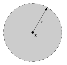
unit circle	open unit ball	closed unit ball

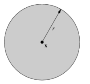1-dim manifold	2-dim manifold	non-manifold, which is indeed a manifold with (closed) boundary

As we shown in the previous section, a unit circle is a 1-dimensional manifold. We can similarly show that an open unit ball is a 2-dimensional manifold.

However, a closed unit ball is NOT a manifold since its interior is an open unit ball and its boundary is a unit circle. The circle and the open unit ball do not have the same dimensionality.

For statistical manifolds, consider the following examples. We will discuss more about them in Part II.

1-dim Gaussian with zero mean	$d$-dim Gaussian with zero mean
$ \{ \mathcal{N}(w \|0,s^{-1}) \Big\| s>0 \}$ with precision $s$ under intrinsic parameterization $\tau = s $	$ \{ \mathcal{N}(\mathbf{w} \|\mathbf{0},\mathbf{S}^{-1}) \Big\| \mathrm{vech}^{-1}(\tau) = \mathbf{S} \succ \mathbf{0} \}$ with precision $\mathbf{S}$ under intrinsic parameterization $\tau = \mathrm{vech}(\mathbf{S})$ .
1-dim statistical manifold	$\frac{d(d+1)}{2}$ -dim statistical manifold

References

[1] S.-I. Amari, "Natural gradient works efficiently in learning," Neural computation 10:251–276 (1998).

[2] W. Lin, F. Nielsen, M. E. Khan, & M. Schmidt, "Tractable structured natural gradient descent using local parameterizations," International Conference on Machine Learning (ICML) (2021).

[3] T. Liang, T. Poggio, A. Rakhlin, & J. Stokes, "Fisher-rao metric, geometry, and complexity of neural networks," The 22nd International Conference on Artificial Intelligence and Statistics (PMLR, 2019), pp. 888–896.

[4] J. Martens, "New Insights and Perspectives on the Natural Gradient Method," Journal of Machine Learning Research 21:1–76 (2020).

[5] M. Khan & W. Lin, "Conjugate-computation variational inference: Converting variational inference in non-conjugate models to inferences in conjugate models," Artificial Intelligence and Statistics (PMLR, 2017), pp. 878–887.

[6] W. Lin, F. Nielsen, M. E. Khan, & M. Schmidt, "Structured second-order methods via natural gradient descent," arXiv preprint arXiv:2107.10884 (2021).

[7] K. Osawa, S. Swaroop, A. Jain, R. Eschenhagen, R. E. Turner, R. Yokota, & M. E. Khan, "Practical deep learning with Bayesian principles," Proceedings of the 33rd International Conference on Neural Information Processing Systems (2019), pp. 4287–4299.

[8] D. Wierstra, T. Schaul, T. Glasmachers, Y. Sun, J. Peters, & J. Schmidhuber, "Natural evolution strategies," The Journal of Machine Learning Research 15:949–980 (2014).

[9] S. M. Kakade, "A natural policy gradient," Advances in neural information processing systems 14 (2001).

[10] N. Le Roux, P.-A. Manzagol, & Y. Bengio, "Topmoumoute Online Natural Gradient Algorithm.," NIPS (Citeseer, 2007), pp. 849–856.

[11] T. Duan, A. Anand, D. Y. Ding, K. K. Thai, S. Basu, A. Ng, & A. Schuler, "Ngboost: Natural gradient boosting for probabilistic prediction," International Conference on Machine Learning (PMLR, 2020), pp. 2690–2700.

[12] L. W. Tu, "An introduction to manifolds. Second," New York, US: Springer (2011).

[13] J. M. Lee, Introduction to Riemannian manifolds (Springer, 2018).

Footnotes:

In differential geometry, an intrinsic parametrization is known as a coordinate chart. ↩

Share on

Twitter Facebook LinkedIn

References

- Amari, S.-I. (1998). Natural gradient works efficiently in learning. Neural Computation, 10(2), 251–276.
- Lin, W., Nielsen, F., Khan, M. E., & Schmidt, M. (2021). Tractable structured natural gradient descent using local parameterizations. International Conference on Machine Learning (ICML).
- Liang, T., Poggio, T., Rakhlin, A., & Stokes, J. (2019). Fisher-rao metric, geometry, and complexity of neural networks. The 22nd International Conference on Artificial Intelligence and Statistics, 888–896.
- Martens, J. (2020). New Insights and Perspectives on the Natural Gradient Method. Journal of Machine Learning Research, 21, 1–76.
- Khan, M., & Lin, W. (2017). Conjugate-computation variational inference: Converting variational inference in non-conjugate models to inferences in conjugate models. Artificial Intelligence and Statistics, 878–887.
- Lin, W., Nielsen, F., Khan, M. E., & Schmidt, M. (2021). Structured second-order methods via natural gradient descent. ArXiv Preprint ArXiv:2107.10884.
- Osawa, K., Swaroop, S., Jain, A., Eschenhagen, R., Turner, R. E., Yokota, R., & Khan, M. E. (2019). Practical deep learning with Bayesian principles. Proceedings of the 33rd International Conference on Neural Information Processing Systems, 4287–4299.
- Wierstra, D., Schaul, T., Glasmachers, T., Sun, Y., Peters, J., & Schmidhuber, J. (2014). Natural evolution strategies. The Journal of Machine Learning Research, 15(1), 949–980.
- Kakade, S. M. (2001). A natural policy gradient. Advances in Neural Information Processing Systems, 14.
- Le Roux, N., Manzagol, P.-A., & Bengio, Y. (2007). Topmoumoute Online Natural Gradient Algorithm. NIPS, 849–856.
- Duan, T., Anand, A., Ding, D. Y., Thai, K. K., Basu, S., Ng, A., & Schuler, A. (2020). Ngboost: Natural gradient boosting for probabilistic prediction. International Conference on Machine Learning, 2690–2700.
- Tu, L. W. (2011). An introduction to manifolds. Second. New York, US: Springer.
- Lee, J. M. (2018). Introduction to Riemannian manifolds. Springer.