Part II: Derivation of Natural-gradients
October 04, 2021
Goal (edited: )
This blog post focuses on the derivation of natural-gradients, which are known as Riemannian gradients with the Fisher-Rao metric. We will discuss the following concepts to derive natural-gradients:
- Rimannian steepest direction (i.e., normalized natural gradient)
- The difference between a parameter space and a gradient/vector space
The discussion here is informal and focuses more on intuitions, rather than rigor.
Click to see how to cite this blog post
Motivation
In machine learning, a common derivation of natural-gradients is via a Talyor expansion of the Kullback-Leibler divergence as we will discuss in Part IV. However, the derivation has the following limitations:
- It does not clearly illustrate the difference between a parameter space and a (natural) gradient space.
- It implicitly assumes that the Fisher information matrix (FIM) is non-singular and the parameter space is open.
These limitations become essential when it comes to constrained parameters (i.e., covariance matrix in a Gaussian family). Moreover, a natural gradient (in a gradient space) is invariant (will show in Part III) while a natural-gradient update (in a parameter space) is only linearly invariant (will discuss in Part IV).
We will give an alternative derivation of natural-gradients to emphasize the subtlety.
Euclidean Steepest Direction
Before we discuss natural-gradients, we first revisit Euclidean gradients.
We will show a normalized Euclidean gradient can be viewed as the Euclidean steepest direction. Later, we will generalize the steepest direction in Riemannian cases and show that the Riemannian steepest direction w.r.t. the Fisher-Rao metric is indeed a normalized natural-gradient.
Consider a minimization problem $\min_{\tau \in \mathcal{R}^K } \,\,f(\mathbf{\tau})$ over a parameter space $\mathcal{R}^K$.
Given the smooth scalar function $f(\cdot)$, we can define the (Euclidean) steepest direction at current point $\mathbf{\tau}_0$ as the optimal solution to another optimization problem,
where we assume $\nabla_\tau f(\mathbf{\tau}_0) \neq \mathbf{0}$.
We can express the optimization problem in terms of a directional derivative along vector $\mathbf{v} \in T_{\tau_0} (\mathcal{R}^K)$, where
$T_{\tau_0} (\mathcal{R}^K)=\mathcal{R}^K$ is a gradient space attached at current point $\mathbf{\tau}_0$.
The optimal directional derivative, denoted by $\mathbf{v}_{\text{opt}}$, is the steepest direction.
$$
\begin{aligned}
\min_{\|v\|^2=1   } \lim_{t \to 0} \frac{f(\mathbf{\tau}_0+t\mathbf{v}) - f(\mathbf{\tau}_0) }{t} = ( \nabla_\tau f(\mathbf{\tau}_0) )^T \mathbf{v}
\end{aligned}\tag{1}\label{1}
$$
It is easy to see that the optimal solution of Eq. $\eqref{1}$ is $\mathbf{v}_{\text{opt}}= -\frac{\nabla_\tau f(\mathbf{\tau}_0) }{\|\nabla_\tau f(\mathbf{\tau}_0) \|}$, which is the (Euclidean) steepest direction at point $\mathbf{\tau}_0$.
Note:
In Euclidean cases, there is no difference between parameter space $\mathcal{R}^K$ and (Euclidean) gradient space $T_{\tau_0} (\mathcal{R}^K)=\mathcal{R}^K$ at point $\tau_0$.
Later, we will see that there is a key difference between a parameter space and a gradient space in manifold cases.
Weighted Norm Induced by the Fisher-Rao Metric
Now, we formulate a similar optimization problem like Eq. $\eqref{1}$ in order to generalize the steepest direction at point $\mathbf{\tau}_0$ in a Riemannian manifold.
To do so, we have to define the length of a vector in manifold cases. In
Part III,
we will show that the (standard) length does not preserve under a parameter transformation while the length induced by the Fisher-Rao metric does.
Thanks to the Fisher-Rao metric, we will further show that a natural-gradient is invariant under parameter transformations.
As mentioned at Part I, the FIM $\mathbf{F}$ is positive definite everywhere in an intrinsic parameter space. We can use the FIM to define the length/norm of a vector (e.g., a Riemannian gradient) $\mathbf{v}$ at a point in a manifold via a weighted inner product. We use an intrinsic parameter $\tau_0$ to represent this point. Note that the FIM is evaluated at current point $\tau_0$.
$$
\begin{aligned}
\|\mathbf{v}\|_F := \sqrt{\mathbf{v}^T \mathbf{F}(\tau_0) \mathbf{v}}
\end{aligned}
$$
The positive-definiteness of the FIM is essential since we do not want a non-zero vector to have a zero length.
The distance (and orthogonality) between two vectors at point $\tau_0$ is also induced by the FIM since we can define them by the inner product as
$$
\begin{aligned}
d(\mathbf{v},\mathbf{w}) := \|\mathbf{v}-\mathbf{w}\|_F
\end{aligned}
$$
where vector $\mathbf{v}$ and $\mathbf{w}$ live in the same (vector) space at point $\tau_0$.
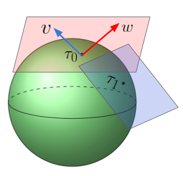
Note:
In the figure,
the vector space at $\tau_0$ is just a $\mathcal{R}^2$ space. In our (intrinsic) settings, we do not care about whether it is embedded in the $\mathcal{R}^3$ space or not.
We will return to embedded (extrinsic) cases when it comes to sub-manifolds and the induced (pull-back) metric.
In manifold cases, we have to distinguish the difference between a point (e.g., parameter array $\tau_0$) and a vector (e.g., Riemannian gradient $\mathbf{v}$ under a parametrization $\tau$).
This difference is crucial to (natural) gradient-based methods in
Part IV.
Warning:
-
We do NOT define how to compute the distance between two points on the manifold, which will be discussed here.
-
We also do NOT define how to compute the distance between a vector at point
$\tau_0$and another vector at a distinct point$\tau_1$, which involves the concept of parallel transport in a curved space. For simplicity, we avoid defining the transport since it involves partial derivatives of the Fisher-Rao metric (closely related to the Christoffel symbols).
Directional Derivatives in a Manifold
As we shown before, the objective function in Eq. $\eqref{1}$ is a directional derivative in Euclidean cases.
The next step is to generalize the concept of directional derivatives in a manifold.
Recall that a manifold should be locally like a vector space under intrinsic parameterization $\mathbf{\tau}$.
Using this parameterization, consider an optimization problem $\min_{\tau \in \Omega_\tau } f(\mathbf{\tau})$, where the parameter space $\Omega_\tau$ is determined by the choice of a parameterization and the manifold. Recall that we have a local vector space structure in $\Omega_\tau$ if we parametrize the manifold with an intrinsic parameterization.
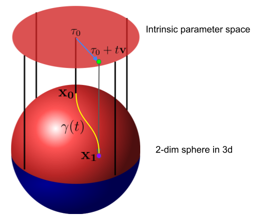
Therefore, we can similarly define a directional derivative1 at $\mathbf{\tau}_0$ along Riemannian vector2 $\mathbf{v}$ as $\lim_{t \to 0} \frac{f(\mathbf{\tau}_0+t\mathbf{v}) - f(\mathbf{\tau}_0) }{t}$, where $t$ is a scalar real number. The main point is that $\mathbf{\tau}_0+t\mathbf{v}$ stays in the parameter space $\Omega_\tau$ thanks to the local vector space structure.
Recall that we allow a small perturbation $E$ around $\tau_0$ contained in parameter space $\Omega_\tau$ (i.e., $E \subset \Omega_\tau$) since $\mathbf{\tau}$ is an intrinsic parameterization.
Therefore, when $|t|$ is small enough, $\mathbf{\tau}_0+t\mathbf{v} $ stays in the parameter space and $f(\mathbf{\tau}_0+t\mathbf{v})$ is well-defined.
Note that we only require $\mathbf{\tau}_0+t\mathbf{v} \in \Omega_\tau$ when $|t|$ is small enough. This is possible since a line segment $ \mathbf{\tau}_0+t\mathbf{v} \in E$ and $E \subset \Omega_\tau$.
Technically, this is because $\Omega_\tau$ is an open set in $\mathcal{R}^K$, where $K$ is the number of entries of parameter array $\tau$.
Under intrinsic parameterization $\mathbf{\tau}$, the directional derivative remains the same as in the Euclidean case thanks to the local vector space structure in $\Omega_\tau$.
$$\begin{aligned} \lim_{t \to 0} \frac{f(\mathbf{\tau}_0+t\mathbf{v}) - f(\mathbf{\tau}_0) }{t} = ( \nabla_\tau f(\mathbf{\tau}_0))^T \mathbf{v}. \end{aligned}$$
Note:
-
$\mathbf{\tau}_0+t\mathbf{v}$stays in the parameter space$\Omega_\tau$when scalar$|t|$is small enough. -
vector
$\mathbf{v}$stays in the tangent vector space$T_{\tau_0} (\Omega_\tau)$at current point$\tau_0$. -
In K-dimensional manifold cases, we have
$\Omega_\tau \subset T_{\tau_0} (\Omega_\tau)=\mathcal{R}^K$. This is the key difference between intrinsic parameter space$\Omega_\tau$and tangent space$T_{\tau_0} (\Omega_\tau)$as illustrated by the following figure.

The following example illustrates directional derivatives in manifold cases.
Valid case: (click to expand)
Invalid case: (click to expand)
Riemannian Steepest Direction
Recall that we have defined the length of a Riemannian vector and directional derivatives in a manifold. Now, we can introduce the Riemannian steepest direction (Absil et al., 2009) . We will use this to define/compute natural-gradients.
By choosing an intrinsic parameterization $\mathbf{\tau}$, a minimization problem over a manifold $\mathcal{M}$ can be translated as
$\min_{\tau \in \Omega_\tau } f(\mathbf{\tau})$ over parameter space $\Omega_\tau$. Recall that $\Omega_\tau$ has a local vector-space structure.
Assuming $\nabla_\tau f(\mathbf{\tau}_0) \neq \mathbf{0}$, we define the Riemannian steepest direction as the
optimal solution to the following new optimization problem. The optimization problem is expressed in terms of a
directional derivative along Riemannian vector $\mathbf{v} \in T_{\tau_0} (\Omega_\tau)$, where $T_{\tau_0}
(\Omega_\tau) = \mathcal{R}^K$ is a vector space attached at current point $\mathbf{\tau}_0$.
$$
\begin{aligned}
\min_{ {\color{red} \|v\|_{F}^2=1} } ( \nabla_\tau f(\mathbf{\tau}_0) )^T  \mathbf{v}
\end{aligned} \tag{2}\label{2}
$$
The optimal solution of Eq. $\eqref{2}$ is $\mathbf{v}_{\text{opt}}= -\frac{ \mathbf{F}^{-1}(\mathbf{\tau}_0) \nabla_\tau f(\mathbf{\tau}_0) }{\| \mathbf{F}^{-1}(\mathbf{\tau}_0)\nabla_\tau f(\mathbf{\tau}_0) \|_F}$ (click to see the derivation)
Definition of Natural-gradients
Given a scalar function $f(\mathbf{\tau})$ with an intrinsic parameter $\tau$, we define a (un-normalized) Riemannian gradient as $ \mathbf{F}_\tau^{-1}(\mathbf{\tau}) \nabla_\tau f(\mathbf{\tau})$, where we denote the corresponding (un-normalized) Euclidean gradient by $\nabla_\tau f(\mathbf{\tau})$.
In machine learning, we often use a learning-rate to control the length of a gradient instead of normalizing its length.
Since we use the Fisher-Rao metric $\mathbf{F}$, a Riemannian gradient is also known as a natural gradient.
Now, we give an example to illustrate the definition.
Example: Univariate Gaussian
Consider the following scalar function
$$ \begin{aligned} f(\tau):= E_{q(w|\tau)} [ w^2 + \log q(w|\tau) ] = \mu^2 + \frac{1}{s} + \frac{1}{2} \log(s) - \frac{1}{2}(1+\log(2\pi)) \end{aligned} $$where$q(w|\tau)= \mathcal{N}(w|\mu,s^{-1})$is a Gaussian family with mean$\mu$, variance$s^{-1}$, intrinsic parametrization$\tau=(\mu,s)$, and parameter space$\Omega_\tau=\{(\mu,s)|\mu \in \mathcal{R},s>0 \}$.The FIM of Gaussian $q(w|\tau)$ under this parametrization is
$$
\begin{aligned}
\mathbf{F}_\tau (\tau)  = -E_{q(w|\tau)} [ \nabla_\tau^2 \log q(w|\tau) ]
=
\begin{bmatrix}
s & 0 \\
0 & \frac{1}{2s^2}
\end{bmatrix}
\end{aligned}
$$
Now, we consider a member $\tau_0=(0.5,1)$ in the Gaussian family. The Euclidean gradient is$$ \begin{aligned} \nabla_\tau f(\tau_0) = \begin{bmatrix} 2 \mu \\ -\frac{1}{s^2} +\frac{1}{2s} \end{bmatrix}_{\tau=\tau_0} =\begin{bmatrix} 1 \\ -\frac{1}{2} \end{bmatrix} \end{aligned} $$The natural/Riemannian gradient is$$ \begin{aligned} \mathbf{F}_\tau^{-1} (\tau_0) \nabla_\tau f(\tau_0) = \begin{bmatrix} 2 \mu s^{-1} \\ ( -\frac{1}{s^2} +\frac{1}{2s} ) (2s^2) \end{bmatrix}_{\tau=\tau_0} =\begin{bmatrix} 1 \\ -1 \end{bmatrix} \end{aligned} $$
Example: Multivariate Gaussian (click to expand)
Riemannian Gradients as Tangent Vectors (Optional)
In the previous section, we only consider Riemannian vectors/gradients under a parametrization $\tau$. Now, we will discuss abstract Riemannian vectors without specifying a parametrization (Tu, 2011). This concept is often used to show the invariance of Riemannian gradients, which will be discussed in Part III.
A Riemannian gradient denoted by $\mathbf{v}(\tau)$ is indeed a tangent vector $\mathbf{v}$ of a smooth curve on the manifold under the parametrization $\tau$. The set of tangent vectors evaluated at $\mathbf{\tau}_0$ is called the tangent space at the corresponding point. We will illustrate this by an example.
Let’s denote the unit sphere by $\mathcal{M}$, where we set the origin to be the center of the sphere. Point $\mathbf{x_0}=(0,0,1)$ is the north pole.
We use the following parameterization, where the top half of the sphere can be locally expressed as $\{(\tau_x,\tau_y,\sqrt{1-\tau_x^2-\tau_y^2})| \tau_x^2 + \tau_y^2 <1 \}$ with parameter $\mathbf{\tau}=(\tau_x,\tau_y)$.
Under parametrization $\mathbf{\tau}$, we have the following parametric representations.
| Parametric representation | |
|---|---|
| North pole $\mathbf{x_0}$ | $\mathbf{\tau}_0=(0,0)$ |
| Intrinsic parameter space | red space $\Omega_\tau:=\{ (\tau_x,\tau_y)| \tau_x^2 + \tau_y^2 <1 \}$ |
| Tangent space at $\mathbf{x_0}$ | green space $\mathcal{R}^2$ at $\mathbf{\tau}_0$ |
| Yellow curve from $\mathbf{x_0}$ to $\mathbf{x_1}$ | blue line segment from $\mathbf{\tau}_0$ to $\mathbf{\tau}_0+t\mathbf{v}(\tau_0)$ |
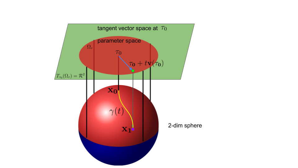
Note that $\tau_0$ is a parameter array, which is a representation of a point $\mathbf{x}_0$ while $\mathbf{v}(\tau_0)$ is a Riemannian gradient, which is a representation of the tangent vector of curve $\gamma$ at point $\mathbf{x}_0$.
Warning: Be aware of the differences shown in the table.
| parametric representation of | supported operations | distance discussed in this post | |
|---|---|---|---|
$\mathcal{R}^2$ (vector/natural-gradient) space |
tangent vector space at $\mathbf{x}_0$ |
real scalar product, vector addition | defined |
$\Omega_\tau$ (point/parameter) space |
top half of the manifold | local scalar product, local vector addition | undefined |
Under intrinsic parametrization $\tau$, we have $\Omega_\tau \subset \mathcal{R}^2$. Thus, we can perform this operation in $\Omega_\tau$ space: $\tau_0 +t\mathbf{v}(\tau_0) \in \Omega_\tau$ when scalar $|t|$ is small enough. Note that we only define the distance between two (Riemannian gradient) vectors in the tangent space. The distance between two points in the $\Omega_\tau$ space is undefined in this post.
Parameterization-free Representation
The tangent vector $\mathbf{v}$ at point $\mathbf{x_0}$ can be viewed as the tangent direction of a (1-dimensional) smooth curve $\gamma(t) \in \mathcal{M}$, where $\gamma(0)=\mathbf{x_0}$ and $\frac{d {\gamma}(t) }{d t} \Big|_{t=0}=\mathbf{v}$ and the support of $\gamma(t)$ denoted by $\mathbf{I}$ is an open interval in $\mathcal{R}^1$ containing 0.
Since a curve $\gamma(t)$ is a geometric object, its tangent direction is also a geometric object.
Note that a parametrization is just a representation of a geometric object.
Thus, the tangent direction should be a parameterization-free representation of vector $\mathbf{v}$.
For example, in physics, the concept of parameterization-free representation means that a law of physics should be independent of any (reference) coordinate system chosen by an observer.
Readers who are not familiar with this abstract concept can safely skip this since in practice, we will always choose a parametrization when it comes to computation. A key takeaway is that a geometric property (i.e., length of a vector) should be invariant to the choice of valid parametrizations.
Parameterization-dependent Representation
Given intrinsic parametrization $\tau$, we can define the parametric representation of the curve denoted by ${\gamma}_\tau(t)$, where the domain is $\mathbf{I}_\tau \subset \mathcal{R}^1$.
The parametric representation of vector $\mathbf{v}$ is defined as $\mathbf{v}(\mathbf{\tau}_0):= \frac{d {\gamma}_{\tau}(t) }{d t} \Big|_{t=0}$, where ${\gamma}_{\tau}(0)=\tau_0$.
Example
Consider the yellow curve in the figure $\gamma(t) = (t v_{x}, t v_{y}, \sqrt{1 - t^2(v_{x}^2 + v_{y}^2) } ) \in \mathcal{M} $ and the blue line segment
${\gamma}_{\tau}(t)= (t v_{x} , t v_y ) \in \Omega_\tau $, where$|t|$must be small enough.The parametric representation of the vector is
$\mathbf{v}(\mathbf{\tau}_0):= \frac{d {\gamma}_\tau(t) }{d t} \Big|_{t=0}=(v_x,v_y)$.
A Riemannian gradient $\mathbf{v}(\mathbf{\tau}_0)$ can be viewed as a parametric representation of tangent vector $\mathbf{v}$ as shown below.
Consider a smooth scalar function defined on the manifold $h: \mathcal{M} \to \mathcal{R}$. In the unit sphere case, consider
$h(\mathbf{z})$subject to$\mathbf{z}^T \mathbf{z}=1$. Under parameterization $\mathbf{\tau}$, we can locally re-expressed the function as$h_\tau(\mathbf{\tau}):=h( (\tau_x,\tau_y,\sqrt{1-\tau_x^2-\tau_y^2}) )$where$\tau \in \Omega_\tau$.By the definition of a directional derivative, the following identity holds for any smooth scalar function $h$:
$[\nabla h_\tau(\mathbf{\tau}_0)]^T \mathbf{v}(\mathbf{\tau}_0) =\frac{d h_\tau({\gamma}_\tau(t)) }{d t} \Big|_{t=0}$, where $h_\tau$ is the parametric representation of $h$ . Note that$(h_\tau \circ {\gamma}_\tau) (t)$is a function defined from$\mathbf{I}_\tau $to $\mathcal{R}^1$, where domain$\mathbf{I}_\tau \subset \mathcal{R}^1$.The key observation:
Function
$(h_\tau \circ {\gamma}_\tau) (t)$becomes a standard real-scalar function thanks to parametrization $\tau$. Thus, we can safely use the standard chain rule.By the chain rule, we have
$\frac{d h_\tau({\gamma}_\tau(t)) }{d t} \Big|_{t=0}=[\nabla h_\tau(\mathbf{\tau}_0)]^T \frac{d {\gamma}_\tau(t) }{d t} \Big|_{t=0}$, where${\gamma}_\tau(0)=\tau_0$. Thus,$\mathbf{v}(\mathbf{\tau}_0) = \frac{d {\gamma}_\tau(t) }{d t} \Big|_{t=0}$since (Euclidean gradient)$\nabla h_\tau(\mathbf{\tau}_0)$is an arbitrary vector in $\mathcal{R}^2$ and$\tau$is a 2-dim parameter array.In summary, a Riemannian gradient
$\mathbf{v}(\mathbf{\tau}_0)$can be viewed as a parametric representation of the tangent vector of curve$\gamma(t)$at$\mathbf{x}_0$since${\gamma}_\tau(t)$is the parametric representation of$\gamma(t)$.
(Riemannian) Gradient Space has a Vector-space Structure
We can similarly define vector additions and real scalar products in a tangent vector space by using the tangent direction of a curve on the manifold with/without a parameterization.
A key takeaway is that a vector space structure is an integral part of a tangent vector space. On the other hand, we have to use an intrinsic parametrization $\tau$ to artificially create a local vector space structure in parameter space $\Omega_\tau$.
We will discuss more about this difference in Part IV.
References
- Absil, P.-A., Mahony, R., & Sepulchre, R. (2009). Optimization algorithms on matrix manifolds. Princeton University Press.
- Tu, L. W. (2011). An introduction to manifolds. Second. New York, US: Springer.
Footnotes:
-
For simplicity, we avoid defining a (coordinate-free) covariant derivative, which induces parallel transport. Given a smooth scalar field/function on a manifold, a coordinate representation of the covariant derivative remains the same as the Euclidean case. Note that the standard coordinate derivative is identical to the coordinate representation of the covariant derivative when it comes to a scalar field. ↩
-
A Riemannian gradient is a coordinate representation of a contravariant vector (A.K.A. a Riemannian vector) while a Euclidean gradient is a coordinate representation of a covariant vector (A.K.A. a Riemannian covector). We will discuss their transformation rules in Part III. ↩