Warning: working in Progress (incomplete)

Goal (edited: 07-Jan-23)

This blog post should help readers to understand natural-gradient descent and Riemannian gradient descent. We also discuss some invariance property of natural-gradient descent, Riemannian gradient descent, and Newton’s method.

We will give an informal introduction with a focus on high level of ideas.

@misc{lin2021NGDblog04,
  title = {Introduction to Natural-gradient Descent: Part IV},
  author = {Lin, Wu and Nielsen, Frank and Khan, Mohammad Emtiyaz and Schmidt, Mark},
  url = {https://informationgeometryml.github.io/year-archive/}, 
  howpublished = {\url{https://informationgeometryml.github.io/posts/2021/11/Geomopt04/}},
  year = {2021},
  note = {Accessed: 2021-11-15}
}

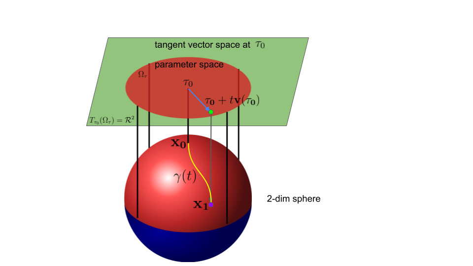
Two kinds of Spaces

We will discuss (Riemannian) gradient spaces and parameter spaces for gradient-based updates.

As we disucssed in Part II, the parameter space ${\mathrm{\Omega }}_{\tau }$ and the tangent space denoted by $T_{{\tau }_0}\mathcal{M}$ at point ${\tau }_0$ are two distinct spaces. Given intrinsic parametrization $\tau$, the tangent space is a (complete) vector space and $T_{{\tau }_0}\mathcal{M}={\mathcal{R}}^K$ while the parameter space ${\mathrm{\Omega }}_{\tau }$ is like a local vector space in ${\mathcal{R}}^K$, where $K$ is the dimension of the manifold. In other words, ${\mathrm{\Omega }}_{\tau }$ is often an open (proper) subset of ${\mathcal{R}}^K$.

In manifold cases, we have to explicitly distinguish the difference between the representation of a point (parameter) and a vector (Riemannian gradient). These two spaces are different in many aspects such as the domain and the distance. Mathematically speaking, a (Riemannian) gradient space is much simpler and nicer than a parameter space.

Natural-gradient Descent in an Intrinsic Parameter Space

Using intrinsic parametrization $\tau$, we can perform a natural-gradient update known as natural-gradient descent (NGD) [1] when we use the Fisher-Rao metric.

where ${\hat{\mathbf{g}}}_{{\tau }_k}:=-\mathbf{v}({\tau }_k)$ is a natural gradient evaluated at point ${\tau }_k$ and $\alpha :=t>0$ is a step-size.

This update in Eq. $\text{(1)}$ is inspired by the standard linear update in the tangent vector space (see the green space in the above figure). By choosing an intrinsic parametrization, this update is also valid in the parameter space¹ (see the red space in the above figure) as long as the step-size is small enough.

The update in the parameter space is valid since the parameter space ${\mathrm{\Omega }}_{\tau }$ has a local vector-space structure thanks to the use of an intrinsic parametrization. However, when ${\mathrm{\Omega }}_{\tau }$ is a proper subset of $T_{{\tau }_k}\mathcal{M}$ (i.e., ${\mathrm{\Omega }}_{\tau }\ne T_{{\tau }_k}\mathcal{M}$), the update in Eq. $\text{(1)}$ is valid only when the step-size $\alpha$ is small enough so that ${\tau }_{k+1}\in {\mathrm{\Omega }}_{\tau }$.

Natural-gradient Descent is Linearly Invariant

Recall that in Part III, we have shown that natural gradients are invariant under any intrinsic parameter transformation. The parameter transformation can be non-linear.

It is natural to expect that natural-gradient descent has a similar property. Unfortunately, natural-gradient descent is only invariant under an intrinsic linear transformation. Note that Newton’s method is also linearly invariant while Euclidean gradient descent is not.

Let’s consider the following (scalar) optimization problem on a smooth manifold $\mathcal{M}$ with the Fisher-Rao metric $F$. $$\begin{array}{}\text{(2)}& \begin{array}{r}\underset{x\in \mathcal{M}}{min}h(x)\end{array}\end{array}$$

Note that $\mathcal{M}$ in general does not have a vector-space structure. We has to artificially choose an intrinsic parameterization $\tau$ so that the parameter space ${\mathrm{\Omega }}_{\tau }$ at least has a local vector-space structure. The problem in $\text{(2)}$ can be re-expressed as below. $$\begin{array}{r}\underset{\tau \in {\mathrm{\Omega }}_{\tau }}{min}{h}_{\tau }(\tau )\end{array}$$ where $h_{\tau }$ is the parameter representation of the smooth function $h$.

Natural gradient descent in this parameter space ${\mathrm{\Omega }}_{\tau }$ is $$\begin{array}{}\text{(3)}& \begin{array}{r}{\tau }_{k+1}\leftarrow {\tau }_k-\alpha {\hat{\mathbf{g}}}_{{\tau }_k}\end{array}\end{array}$$ where ${\mathbf{F}}_{\lambda }$ is the FIM, natural gradient is ${\hat{\mathbf{g}}}_{{\tau }_k}:=[{\mathbf{F}}_{\tau }({\tau }_k){]}^{-1}{\mathrm{\nabla }}_{\tau }{h}_{\tau }({\tau }_k)$ and the step-size $\alpha$ is small enough so that ${\tau }_{k+1}\in {\mathrm{\Omega }}_{\tau }$.

Consider another intrinsic parameterization $\lambda$ so that $\lambda =\mathbf{U}\tau$, where $\mathbf{U}$ is a constant (square) invertible matrix. For simplicity, we further assume ${\mathrm{\Omega }}_{\lambda }=\{\mathbf{U}\tau |\tau \in {\mathrm{\Omega }}_{\tau }\}$, where ${\mathrm{\Omega }}_{\lambda }$ is the parameter space of $\lambda$.

Natural gradient descent in this parameter space ${\mathrm{\Omega }}_{\lambda }$ is $$\begin{array}{}\text{(4)}& \begin{array}{r}{\lambda }_{k+1}\leftarrow {\lambda }_k-\alpha {\hat{\mathbf{g}}}_{{\lambda }_k}\end{array}\end{array}$$ where ${\hat{\mathbf{g}}}_{{\lambda }_k}:=[{\mathbf{F}}_{\lambda }({\lambda }_k){]}^{-1}{\mathrm{\nabla }}_{\lambda }{h}_{\lambda }({\lambda }_k)$ and the cost function is $h_{\lambda }(\lambda )=h_{\tau }(\tau (\lambda ))$.

Recall that we have the transformation rule for natural gradients as $$\begin{array}{r}{\hat{\mathbf{g}}}_{\tau }=\mathbf{Q}{\hat{\mathbf{g}}}_{\lambda }\end{array}$$ where $Q_{ji}=\frac{\partial {\tau }^j(\lambda )}{\partial {\lambda }^i}$.

We can verify that $\mathbf{Q}={\mathbf{U}}^{-1}$. Notice that ${\tau }_0={\mathbf{U}}^{-1}{\lambda }_0$ by construction. The update in $\text{(3)}$ at iteration $k=1$ then can be re-expressed as $$\begin{array}{r}{\tau }_1\leftarrow {\tau }_0-\alpha {\hat{\mathbf{g}}}_{{\tau }_0}={\mathbf{U}}^{-1}{\lambda }_0-\alpha {\mathbf{U}}^{-1}{\hat{\mathbf{g}}}_{{\lambda }_0}={\mathbf{U}}^{-1}{\lambda }_1\end{array}$$

When $\alpha$ is small enough, we have ${\tau }_1\in {\mathrm{\Omega }}_{\tau }$ and ${\lambda }_1\in {\mathrm{\Omega }}_{\lambda }$. It is easy to show that ${\tau }_k={\mathbf{U}}^{-1}{\lambda }_k$ by induction. Therefore, updates in $\text{(3)}$ and $\text{(4)}$ are equivalent.

Riemannian Gradient Descent and its (Non-linear) Invariance

Now we discuss a gradient-based method that is invariant to any intrinsic parameter transformation.

As mentioned before, a manifold in general does not have a vector-space structure. We has to artificially choose an intrinsic parameterization $\tau$, which gives rise to a parametrization-dependence. Therefore, it will be ideal if a gradient-based method does not dependent on the choice of intrinsic parametrizations.

We will first introduce the concept of a (one-dimensional) geodesic $\gamma (t)$, which is the “shortest curve” on a manifold with a Riemannian metric (i.e., the Fisher-Rao metric). Recall that in Part II we only define a distance between two Riemannian gradients evaluated at the same point. We can use the length of the shortest geodesic to define the distance between two points on the manifold. In statistics, the distance induced by a geodesic with the Fisher-Rao metric is known as the Rao distance [2]. This is known as the boundary value problem (BVP) of a geodesic. The boundary conditions are specified by a starting point and an end point on the manifold. To solve this problem, we often solve an easier problem, which is known as the initial value problem (IVP) of a geodesic. The initial conditions are specified by a starting point and an initial Riemannian gradient/velocity.

We will only consider the IVP of a geodesic for simplicity. Consider an intrinsic parametrization $\tau$, where ${\gamma }_{\tau }(t)$ is the parameter representation of the geodesic. To specify a geodesic, we need to provide a starting point ${\tau }_0$ on the manifold and a Riemannian gradient ${\mathbf{v}}_{{\tau }_0}$ evluated at point ${\tau }_0$. The geodesic is the solution of a system of second-order non-linear ordinary differential equations (ODE) with the following initial conditions. $$\begin{array}{r}{\gamma }_{\tau }(0)={\tau }_0;\frac{d{\gamma }_{\tau }(t)}{dt}{|}_{t=0}={\mathbf{v}}_{{\tau }_0}\end{array}$$ where the geodesic is uniquely determined by the initial conditions and ${\mathbf{I}}_{\tau }$ is the domain of the parametric geodesic curve. We assume 0 is contained in the domain for simplicity.

For a geodesically complete manifold, the domain of the geodesic is the whole space ${\mathbf{I}}_{\tau }=\mathcal{R}$. We will only consider this case in this post.

To avoid explicitly writing down the differential equations of a geodesic² (i.e., Christoffel symbols or connection 1-form in a section), researchers refer to it as the manifold exponential map. Given an intrinsic parametrization $\tau$, the map at point ${\tau }_0$ is defined as $$\begin{array}{rl}{\mathrm{Exp}}_{{\tau }_0}:T_{{\tau }_0}\mathcal{M}& \mapsto \mathcal{M}\\ {\mathbf{v}}_{{\tau }_0}& \mapsto {\gamma }_{\tau }(1)\text{s.t.}{\gamma }_{\tau }(0)={\tau }_0;\frac{d{\gamma }_{\tau }(t)}{dt}{|}_{t=0}={\mathbf{v}}_{{\tau }_0}\end{array}$$ where $t$ is fixed to be 1 and ${\tau }_0$ denotes the initial point under parametrization $\tau$.

Now, we can define a Riemannian gradient method. Under intrinsic parametrization $\tau$ of a manifold, (exact) Riemannian gradient descent (RGD) is defined as

where ${\tau }_{k+1}$ always stays on the manifold thanks to the exponential map since ${\hat{\mathbf{g}}}_{{\tau }_k}$ is in the domain of the exponential map.

The invariance of this update is due to the uniqueness of the geodesic and the invariance of the Euler-Lagrange equation. We will not discuss this further in this post to avoid complicated derivations. We will cover this in future posts about calculus of variations.

Although Riemannian gradient descent is nice, the exponential map or the geodesic often has a high computational cost and does not admit a closed-form expression.

Many faces of Natural-gradient Descent

Natural-gradient Descent as Inexact Riemannian Gradient Descent

Natural-gradient descent can be derived from a first-order (linear) approximation of the geodesic, which implies that natural-gradient descent is indeed an inexact Riemannian gradient update. Natural-gradient descent is linearly invariant due to the approximation.

Consider a first-order Taylor approximation at $t=0$ of the geodesic shown below. $$\begin{array}{r}{\gamma }_{\tau }(t)\approx {\gamma }_{\tau }(0)+\frac{d{\gamma }_{\tau }(t)}{dt}{|}_{t=0}(t-0)\end{array}$$

Recall that the exponential map is defined via the geodesic ${\gamma }_{\tau }(1)$. We can use this approximation of the geodesic to define a new map (A.K.A. the Euclidean retraction map) as shown below. $$\begin{array}{r}{\mathrm{Ret}}_{{\tau }_0}({\mathbf{v}}_{{\tau }_0}):={\gamma }_{\tau }(0)+\frac{d{\gamma }_{\tau }(t)}{dt}{|}_{t=0}(1-0)={\tau }_0+{\mathbf{v}}_{{\tau }_0}\end{array}$$

Therefore, an inexact Riemannian gradient update with this new map is defined as $$\begin{array}{r}{\tau }_{k+1}\leftarrow {\mathrm{Ret}}_{{\tau }_k}(-\alpha {\hat{\mathbf{g}}}_{{\tau }_k})={\tau }_k-\alpha {\hat{\mathbf{g}}}_{{\tau }_k}\end{array}$$ which recovers natural-gradient descent.

Natural-gradient Descent as Unconstrained Proximal-gradient Descent

In this section, we will make an additional assumption:

As we mentioned before, the distances in the gradient space and the parameter space are defined differently. In the previous section, we use the geodesic to define the distance between two points in a parameter space.

We could also use other “distances” denoted by $\mathrm{D}(.,.)$ (i.e., Kullback–Leibler divergence) [3] to define the length between two points in a parameter space.

In the following section, we assume $p(w|\mathbf{y})$ and $p(w|{\tau }_k)$ are two members in a parameteric distribution family $p(w|\tau )$ indexed by $\mathbf{y}$ and ${\tau }_k$, respectively.

We define a class of f-divergence in this case. Note that a f-divergence can be defined in a more general setting.

Csiszar f-divergence

Let $f:(0,+\mathrm{\infty })\mapsto \mathcal{R}$ be a smooth scalar function satisfying all the following conditions.

• convex in its domain
• $f(1)=0$
• $\ddot{f}(1)=1$

A f-divergence for a parametric family $p(w|\tau )$ is defined as $$\begin{array}{r}{\mathrm{D}}_f(\mathbf{y},{\tau }_k):=\int f(\frac{p(w|\mathbf{y})}{p(w|{\tau }_k)})p(w|{\tau }_k)dw.\end{array}$$ Thanks to Jensen’s inequality, a f-divergence is always non-negative as
$$\begin{array}{r}{\mathrm{D}}_f(\mathbf{y},{\tau }_k)\ge f(\int \frac{p(w|\mathbf{y})}{p(w|{\tau }_k)}p(w|{\tau }_k)dw)=f(\int p(w|\mathbf{y})dw)=f(1)=0.\end{array}$$

The KL divergence is a f-divergence where $f(t)=-\log (t)$.

Proximal-gradient descent

Given such a “distance” $\mathrm{D}(\mathbf{y},{\tau }_k)$, we could perform an unconstrained proximal-gradient update as $$\begin{array}{r}{\tau }_{k+1}\leftarrow \arg \underset{\mathbf{y}\in {\mathcal{R}}^K}{min}\{⟨{\mathbf{g}}_{{\tau }_k},\mathbf{y}⟩+\frac{1}{\alpha }\mathrm{D}(\mathbf{y},{\tau }_k)\}\end{array}$$ where ${\mathbf{g}}_{{\tau }_k}$ is a Eulcidean gradient and the parameter space ${\mathrm{\Omega }}_{\tau }$ is unconstrained.

By the claim, when $\mathrm{D}(\mathbf{y},{\tau }_k)$ is the second-order Taylor approximation of a f-divergence ${\mathrm{D}}_f(\mathbf{y},{\tau }_k)$ at $\mathbf{y}={\tau }_k$, the unconstrained proximal-gradient update can be re-expressed as $$\begin{array}{r}{\tau }_{k+1}\leftarrow \arg \underset{y\in {\mathcal{R}}^K}{min}\{⟨{\mathbf{g}}_{{\tau }_k},\mathbf{y}⟩+\frac{1}{2\alpha }(\mathbf{y}-{\tau }_k{)}^T{\mathbf{F}}_{\tau }({\tau }_k)(\mathbf{y}-{\tau }_k)\}\end{array}$$

It is easy to see that we can obtain the following natural-gradient update from the above expression. $$\begin{array}{r}{\tau }_{k+1}\leftarrow {\tau }_k-\alpha \underset{={\hat{\mathbf{g}}}_{{\tau }_k}}{\underbrace{{\mathbf{F}}_{\tau }^{-1}({\tau }_k){\mathbf{g}}_{{\tau }_k}}}\end{array}$$

In Part V , we will show that $\mathrm{D}(y,{\tau }_k)$ can also be an exact KL divergence when $p(w)$ is an exponential family. Under a particular parametrization, natural-gradient descent also can be viewed as (unconstrained) mirror descent.

Natural-gradient Descent in Non-intrinsic Parameter Spaces

As mentioned in Part I, an intrinsic parametrization creates a nice parameter space (e.g., a local vector space structure) and guarantees a non-singular FIM. We now discuss issues when it comes to natural-gradient descent over non-intrinsic parametrizations including overparameterization.

1. We may not have a local vector space structure in a non-intrinsic parameter space. Therefore, natural-gradient descent in this parameter space is pointless since the updated parameter will leave the parameter space. Indeed, the FIM could also be ill-defined in such cases. We will illustrate this by examples.

   Bernoulli Example: Invalid NGD (click to expand)

   Consider Bernoulli family $\{\mathcal{I}(w=0){\pi }_0+\mathcal{I}(w=1){\pi }_1|{\pi }_0>0,{\pi }_1>0,{\pi }_0+{\pi }_1=1\}$ with parameter $\tau =({\pi }_0,{\pi }_1)$.

   As we shown in Part I, the FIM is ill-defined due to this eqaulity constraint.

   Moreover, the NGD update will violate the eqaulity constraint.

   Von Mises–Fisher Example: Invalid NGD (click to expand)

   Consider $2$-dimensional Von Mises–Fisher family $\{p(\mathbf{w}|\tau ):=C(\kappa )\exp (\kappa (w_1{\mu }_1+w_2{\mu }_2))|\kappa >0,{\mu }_1^2+{\mu }_2^2=1\}$ with parameter $\tau =(\kappa ,{\mu }_1,{\mu }_2)$, where $C(\kappa )$ is the normalization constant, $\kappa$ is a positive scalar, $\mathbf{w}=(w_1,w_2)$ is a random unit vector defined in a circle, and $\mu =({\mu }_1,{\mu }_2)$ is also a unit vector.

   We can show that the FIM is ill-defined under this parametrization due to this eqaulity constraint.

2. The FIM is singular in a non-intrinsic space. In theory, Moore–Penrose inverse could be used to compute natural-gradients so that natural-gradient descent is linearly invariant in this case. However, Moore–Penrose inverse often has to use the singular value decomposition (SVD) and destroies structures of the FIM. In practice, the iteration cost of Moore–Penrose inverse is very high as illustrated in the following example.
   Example: High iteration cost (click to expand)

   Consider a $d$-dimensional Gaussian mixture family $\{\frac{1}{C}\sum _{k=1}^C\mathcal{N}(w|{\mu }_k,{\mathbf{\Sigma }}_k)|{\mu }_k\in {\mathcal{R}}^d,{\mathbf{\Sigma }}_k\succ \mathbf{0}\}$ with $\tau =\{{\mu }_k,{\mathrm{\Sigma }}_k{\}}_{k=1}^C$.

   If we use the following initialization such that all $C$ components have the same mean ${\mu }_0$ and the same covariance ${\mathbf{\Sigma }}_0$, this family becomes a Gaussian family. In this case, $\tau$ is a non-intrinsic parameterization for a Gaussian family. Note that the FIM is singular under parametrization $\tau$. The iteration cost of natural-gradient descent in this parameter space ${\mathrm{\Omega }}_{\tau }$ will be $O(C^3{d}^6)$ if Moore–Penrose inverse is employed.

   Now, consider an equivalent Gaussian family $\{\mathcal{N}(w|\mu ,\mathbf{\Sigma })|\mu \in {\mathcal{R}}^d,\mathbf{\Sigma }\succ \mathbf{0}\}$ with $\lambda =(\mu ,\mathrm{vech}(\mathbf{\Sigma }))$, where $\lambda$ is an intrinsic parameterization of the Gaussian family and initialized by mean ${\mu }_0$ and covariance ${\mathbf{\Sigma }}_0$.

   As we will show in Part V, the iteration cost of natural-gradient descent in this parameter space ${\mathrm{\Omega }}_{\lambda }$ will be $O(d^3)$ if we exploit structures of the exact non-singular FIM.

3. It is tempting to approximate the singular FIM by an emprical FIM with a scalar damping term and use Woodbury matrix identity to reduce the iteration cost of computing natural-gradients. However, sample-based emprical approximations could be problematic [4]. Moreover, damping introduces an additional tuning hyper-parameter and destories the linear invariance property of natural-gradient descent. Such an approximation should be used with caution.

Euclidean Gradient Descent is NOT (Linearly) Invariant

For simplicity, consider an unconstrained optimization problem. $$\begin{array}{r}\underset{\tau \in {\mathcal{R}}^K}{min}{h}_{\tau }(\tau )\end{array}$$

Euclidean gradient descent (GD) in parametrization $\tau$ is $$\begin{array}{}\text{(5)}& \begin{array}{r}{\tau }_{k+1}\leftarrow {\tau }_k-\alpha {\mathbf{g}}_{{\tau }_k}\end{array}\end{array}$$ where ${\mathbf{g}}_{{\tau }_k}:={\mathrm{\nabla }}_{\tau }{h}_{\tau }({\tau }_k)$ is a Euclidean gradient.

Consider a reparametrization $\lambda$ so that $\lambda =\mathbf{U}\tau$, where $\mathbf{U}$ is a constant (square) invertible matrix. $$\begin{array}{r}\underset{\lambda \in {\mathcal{R}}^K}{min}{h}_{\lambda }(\lambda ):=h_{\tau }({\mathbf{U}}^{-1}\lambda )\end{array}$$

The Euclidean gradient descent (GD) in parametrization $\lambda$ is $$\begin{array}{}\text{(6)}& \begin{array}{r}{\lambda }_{k+1}\leftarrow {\lambda }_k-\alpha {\mathbf{g}}_{{\lambda }_k}\end{array}\end{array}$$ where ${\mathbf{g}}_{{\lambda }_k}:={\mathrm{\nabla }}_{\lambda }{h}_{\lambda }({\lambda }_k)$ is a Euclidean gradient.

Note that Euclidean gradients follow the transformation rule as

$$\begin{array}{r}{\mathbf{g}}_{\tau }^T={\mathbf{g}}_{\lambda }^T\mathbf{J}\end{array}$$ where $J_{ki}:=\frac{\partial {\lambda }^k(\tau )}{\partial {\tau }^i}$

We can verify that $\mathbf{J}=\mathbf{U}$ and ${\mathbf{g}}_{\tau }={\mathbf{U}}^T{\mathbf{g}}_{\lambda }$.

Notice that ${\tau }_0={\mathbf{U}}^{-1}{\lambda }_0$ by construction. The update in $\text{(5)}$ at iteration $k=1$ then can be re-expressed as $$\begin{array}{r}{\tau }_1\leftarrow {\tau }_0-\alpha {\mathbf{g}}_{{\tau }_0}={\mathbf{U}}^{-1}{\lambda }_0-\alpha {\mathbf{U}}^T{\mathbf{g}}_{{\lambda }_0}\ne {\mathbf{U}}^{-1}{\lambda }_1\end{array}$$

It is easy to see that updates in $\text{(5)}$ and $\text{(6)}$ are NOT equivalent. Therefore, Euclidean gradient descent is not invariant.

Newton’s Method is Linearly Invariant

For simplicity, consider an unconstrained convex optimization problem. $$\begin{array}{r}\underset{\tau \in {\mathcal{R}}^K}{min}{h}_{\tau }(\tau )\end{array}$$ where $h_{\tau }(\tau )$ is strongly convex and twice continuously differentiable w.r.t. $\tau$.

Newton’s method under parametrization $\tau$ is $$\begin{array}{r}{\tau }_{k+1}\leftarrow {\tau }_k-\alpha {\mathbf{H}}_{\tau }^{-1}({\tau }_k){\mathbf{g}}_{{\tau }_k}\end{array}$$ where ${\mathbf{g}}_{{\tau }_k}:={\mathrm{\nabla }}_{\tau }{h}_{\tau }({\tau }_k)$ is a Euclidean gradient and ${\mathbf{H}}_{\tau }({\tau }_k):={\mathrm{\nabla }}_{\tau }^2{h}_{\tau }({\tau }_k)$ is the Hessian.

Consider a reparametrization $\lambda$ so that $\lambda =\mathbf{U}\tau$, where $\mathbf{U}$ is a constant (square) invertible matrix. $$\begin{array}{r}\underset{\lambda \in {\mathcal{R}}^K}{min}{h}_{\lambda }(\lambda ):=h_{\tau }({\mathbf{U}}^{-1}\lambda )\end{array}$$ where $h_{\lambda }(\lambda )$ is also strongly convex w.r.t. $\lambda$ due to $\text{(7)}$.

Newton’s method under parametrization $\lambda$ is $$\begin{array}{r}{\lambda }_{k+1}\leftarrow {\lambda }_k-\alpha {\mathbf{H}}_{\lambda }^{-1}({\lambda }_k){\mathbf{g}}_{{\lambda }_k}\end{array}$$ where ${\mathbf{g}}_{{\lambda }_k}:={\mathrm{\nabla }}_{\lambda }{h}_{\lambda }({\lambda }_k)$ is a Euclidean gradient and ${\mathbf{H}}_{\tau }({\lambda }_k):={\mathrm{\nabla }}_{\lambda }^2{h}_{\lambda }({\lambda }_k)$ is the Hessian.

As we discussed in the previous section, Euclidean gradients follow the transformation rule as ${\mathbf{g}}_{\tau }^T={\mathbf{g}}_{\lambda }^T\mathbf{J}$, where $\mathbf{J}=\mathbf{U}$.

Surprisingly, for a linear transformation, the Hessian follows the transformation rule like the FIM as

$$\begin{array}{}\text{(7)}& \begin{array}{rl}{\mathbf{H}}_{\tau }({\tau }_k)& ={\mathrm{\nabla }}_{\tau }({\mathbf{g}}_{{\tau }_k})\\ & ={\mathrm{\nabla }}_{\tau }({\mathbf{J}}^T{\mathbf{g}}_{{\lambda }_k})\\ & ={\mathbf{J}}^T{\mathrm{\nabla }}_{\tau }({\mathbf{g}}_{{\lambda }_k})+\underset{=0}{\underbrace{[{\mathrm{\nabla }}_{\tau }{\mathbf{J}}^T]}}{\mathbf{g}}_{{\lambda }_k}\text{(In linear cases, }\mathbf{J}=\mathbf{U}\text{ is a constant)}\\ & ={\mathbf{J}}^T[{\mathrm{\nabla }}_{\lambda }({\mathbf{g}}_{{\lambda }_k})]\mathbf{J}\\ & ={\mathbf{J}}^T{\mathbf{H}}_{\lambda }({\lambda }_k)\mathbf{J}\end{array}\end{array}$$

Therefore, the direction in Newton’s method denoted by ${\tilde{\mathbf{g}}}_{{\tau }_k}:={\mathbf{H}}_{\tau }^{-1}({\tau }_k){\mathbf{g}}_{{\tau }_k}$ is transformed like natural-gradients in linear cases as

$$\begin{array}{rl}{\tilde{\mathbf{g}}}_{{\tau }_k}& :={\mathbf{H}}_{\tau }^{-1}({\tau }_k){\mathbf{g}}_{{\tau }_k}\\ & =[{\mathbf{J}}^T{\mathbf{H}}_{\lambda }({\lambda }_k)\mathbf{J}{]}^{-1}{\mathbf{g}}_{{\tau }_k}\\ & ={\mathbf{J}}^{-1}{\mathbf{H}}_{\lambda }^{-1}({\lambda }_k){\mathbf{J}}^{-T}[{\mathbf{J}}^T{\mathbf{g}}_{{\lambda }_k}]\\ & ={\mathbf{J}}^{-1}{\mathbf{H}}_{\lambda }^{-1}({\lambda }_k){\mathbf{g}}_{{\lambda }_k}\\ & ={\mathbf{J}}^{-1}{\tilde{\mathbf{g}}}_{{\lambda }_k}\\ & =\mathbf{Q}{\tilde{\mathbf{g}}}_{{\lambda }_k}\end{array}$$ where by the definition we have $\mathbf{Q}={\mathbf{J}}^{-1}$.

The consequence is that Newton’s method like natural-gradient descent is linearly invariant.

The Hessian is not a valid manifold metric

The Hessian ${\mathbf{H}}_{\tau }({\tau }_k)={\mathrm{\nabla }}_{\tau }^2{h}_{\tau }({\tau }_k)$ in general is not a valid manifold metric since it does not follow the transformation rule of a metric in non-linear cases³.

Contrastingly, the FIM is a valid manifold metric. Recall that the FIM can also be computed as ${\mathbf{F}}_{\tau }(\tau )=E_{p(w|\tau )}[-{\mathrm{\nabla }}_{\tau }^2\log p(w|\tau )]$.

We will discuss in Part V, for a special parametrization $\tau$ (known as a natural parametrization) of exponential family, the FIM under this parametrization can be computed as ${\mathbf{F}}_{\tau }(\tau )={\mathrm{\nabla }}_{\tau }^2{A}_{\tau }(\tau )$, where $A_{\tau }(\tau )$ is a strictly convex function.

In the literature, the exponential family with a natural parametrization is known as a Hessian manifold [5], where the FIM under this kind of parametrization is called a Hessian metric. However, a non-linear reparametrization will lead to a non-natural parametrization.

References

[1] S.-I. Amari, "Natural gradient works efficiently in learning," Neural computation 10:251–276 (1998).

[2] C. Atkinson & A. F. S. Mitchell, "Rao’s distance measure," Sankhyā: The Indian Journal of Statistics, Series A 345–365 (1981).

[3] M. E. Khan, R. Babanezhad, W. Lin, M. Schmidt, & M. Sugiyama, "Faster stochastic variational inference using Proximal-Gradient methods with general divergence functions," Proceedings of the Thirty-Second Conference on Uncertainty in Artificial Intelligence (2016), pp. 319–328.

[4] F. Kunstner, P. Hennig, & L. Balles, "Limitations of the empirical Fisher approximation for natural gradient descent," Advances in Neural Information Processing Systems 32:4156–4167 (2019).

[5] H. Shima, The geometry of Hessian structures (World Scientific, 2007).

Footnotes: